ESDEP WG 12
FATIGUE
To gain an understanding of the fatigue behaviour of hollow section joints and the available methods of design.
Lecture 12.1: Basic Introduction to Fatigue
Lecture 12.3: Effect of Workmanship on Fatigue Strength of Longitudinal and Transverse Welds
Lecture 13.1: Application of Hollow Sections in Steel Structures
Lecture 13.2: The Behaviour and Design of Welded Connections between Circular Hollow Sections under Predominantly Static Loading
Lecture 13.3: The Behaviour and Design of Welded Connection between Rectangular Hollow Sections under Predominantly Static Loading
Lecture 12.4.2: The Fatigue Behaviour of Hollow Section Joints (II)
In hollow section joints the stiffness along the intersection of the connected members is generally rather non-uniform, which may result in large peak stresses. The peak stress ranges determine the fatigue behaviour to a large extent.
This lecture describes the basic behaviour and introduces the methods of analysis. Detailed design is presented in Lecture 12.4.2.
The notation of Eurocode 3 [1] has been adopted.
Hollow sections (circular, square and rectangular) are used in many applications subjected to fatigue loading, e.g. cranes, bridges, offshore jacket structures and several applications in mechanical engineering. The phenomenon of fatigue, the factors influencing it, definitions and loading are described in the Lectures 12.1 to 12.3. In these lectures it is shown that the peak stress ranges determine the fatigue life of a particular connection to a large extent.
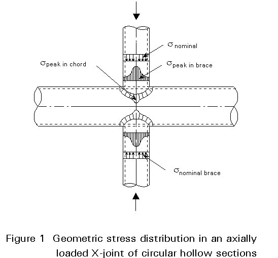
In Lecture 13.1 it is shown that the most economical construction of hollow section structures is obtained by the direct welded connection of hollow section members avoiding stiffeners or gusset plates. In such a connection the stiffness around the intersection is not uniform, resulting in a geometrical non-uniform stress distribution, as shown in Figure 1, for an X-joint of circular hollow sections. This non-uniform stress distribution depends on the type of loading (axial, bending in-plane, bending out-of-plane) and the connection (type and geometry). Thus, many cases exist. For this reason the fatigue behaviour of hollow section joints is generally treated in a different way to that, for example, for welded connections between plates.
The fatigue behaviour can be determined either by Ds-N methods or with a fracture mechanics (F.M.) approach.
The various Ds-N methods are based on experiments resulting in Ds-N graphs with a defined stress range Ds on the vertical axis and the number of cycles N to a specified failure criterion on the horizontal axis. The F.M. approach is based on a fatigue crack growth model. The material crack growth parameters of the model can be determined from standardized small specimens and the influence of the connection geometry is incorporated in the stress intensity factor DK, see Lectures 12.10 to 12.15. This lecture describes the Ds-N methods.
In the Ds-N concepts the stress range and failure criterion have to be defined. Considering the X-joint in Figure 1, "nominal" stresses are shown in the brace members and the peak stresses at the connection, i.e. at the intersection of the brace and chord members.
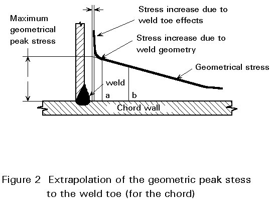
For axial loading, the nominal stresses in the members are defined. However, for bending moments a certain cross-section has to be defined. Considering the peak stress (Figure 2) at the intersection, the peak stress considered has to be defined, since for a certain loading the actual peak stress is determined by:
The local condition at the weld toe depends on the fabrication (welder, welding conditions and welding process). This effect is generally indirectly incorporated in the scatter of the test results. The same applies to the shape of the weld (flat, convex or concave). The fatigue behaviour of fillet welded specimens is sometimes related by factors to that of butt welded specimens.
Initially it was thought that if a geometric (or so-called hot spot) peak stress range is used which takes the global geometry and the loading into account, the fatigue behaviour of all types of joints could be related to one basic Sr-N line. However, the crack propagation not only depends on the actual peak stress range, but on the whole stress pattern. Consequently, the stress gradients also have an influence. At present these stress gradients cannot be incorporated in a proper manner in a concept based on the geometric or hot spot stress range. Furthermore, as will be shown later the thickness also has an influence which is independently taken into account.
In the geometric stress or hot spot stress approach the geometrical stress range is used as the basis for analysis. The geometric hot spot stress (range) is defined as the maximum extrapolated stress (range) to the weld toe, taking the global geometrical effects into account.
The extrapolation is defined in such a way that the effects of the global geometry of the weld (flat, concave, convex) and the condition at the weld toe (angle, undercut) are not included in the geometric stress. Therefore, the first point of extrapolation should be outside the influence area of the weld, see Figure 2.
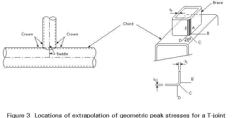
For linear extrapolation, two points are defined at the crown and saddle position of chord and brace [2]. Based on the work of Gurney [3] and Van Delft [4] this first point can be taken at 0,4 (to or t1) with a minimum of 4 mm from the weld toe. The second point is defined depending on the type of hollow sections used (circular or rectangular).
In those cases where the geometric stress distribution is not linear, a quadratic extrapolation is defined with well defined measuring points, see Lecture 12.5.
In some codes it is stated that the principal stress should be extrapolated to the weld toe. However, this has several disadvantages [5]:
In view of the above arguments, extrapolation of stresses perpendicular to the weld toe is favoured.
For a particular loading case and a particular type of joint with a defined geometry, the extrapolated geometric or hot spot stress can be determined from measurements on actual steel specimens or acrylic models or with finite element calculations. However, this is not suitable for design. For this reason the geometric or hot spot peak stresses are related by stress concentration factors to the nominal stress in the member (in most cases the brace) which causes the geometric stress at the intersection of the brace with the chord. For example, for an X-joint without chord loading the stress concentration factor for a particular location (chord, brace; crown or saddle) is defined as:
SCFi.j.k = ![]() (1)
(1)
where
i is the chord or brace
j is the location, e.g. crown or saddle for CHS joints
k is the type of loading
In this way, stress concentration factors can be determined for various load conditions (axial loading, bending in-plane and bending out-of-plane) at various locations, e.g. crown and saddle positions of chord and brace.
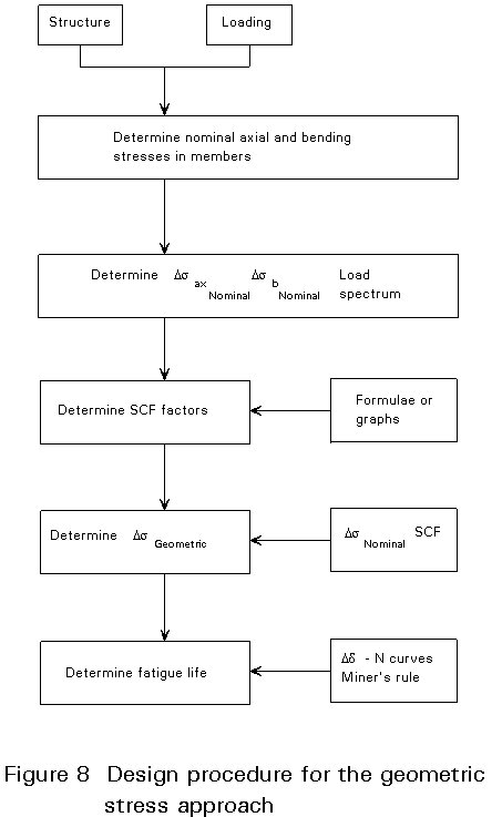
Based on parametric finite element studies, parametric formulae have been developed which give the stress concentration factors for various locations and loading. For a combined loading, the nominal stress ranges of the brace have to be multiplied by the relevant stress concentration factor for that particular location i.j. and the relevant loading case k, e.g:
Ds
i.j.k = Dsaxbrace . SCFaxi.j + Dsbipbrace . SCFbipi.j + Dsbopbrace . SCFbopi.j(2)
This has to be done for the chord and brace (i) at various locations (j), see Figure 3, for a T-joint.
The geometric stresses considered until now are caused by the forces or moments in the brace. But the forces in the chord will also cause stress concentrations at the intersection, although they are considerably smaller. These effects also have to be incorporated. But here the stress concentration factors are related to the nominal stress in the chord. The effect of chord loading on the geometric peak stress in the brace is generally small and can be neglected. For the chord, however, the stress concentration factor can reach values up to 2,5 (see Lecture 12.4.2).
With the method described above, the geometric stress range can be determined for various locations of the chord and the brace considering the relevant loading.
Since the fatigue behaviour depends on the thickness, the maximum geometric or hot spot stress range has to be determined for the chord and the brace considering different thicknesses. Using the Ds-N curve for geometric or hot spot stress, the number of cycles to failure can be determined.
The fatigue life is generally specified as the number of cycles N for stress or strain of a specified character that a given joint sustains before failure of a specified nature occurs.
Various modes of failure can be considered [6], e.g.
Figure 4 shows the relationship between extrapolated, measured geometric stress at a critical location versus the number of cycles. The fatigue life of welded hollow section joints is related to both crack initiation and crack propagation. Their importance depends on the size and type of joint, e.g. the initiation period may cover 10 to 80% of the total fatigue life.
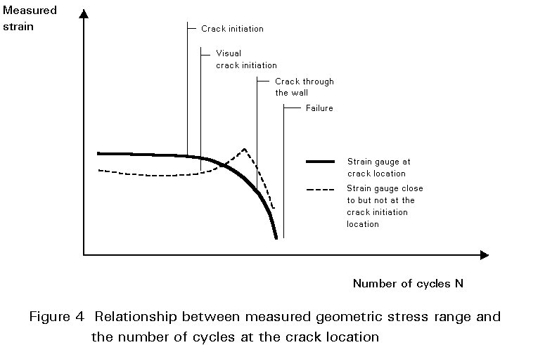
Usually, a crack through the wall is adopted as the failure criterion for hollow section joints, which corresponds to about 80% of the total fatigue life of a joint.
The reason that a lower fatigue strength is found for specimens with larger thicknesses, where specimens have the same geometry and loading and the same geometric stress range but a different size, is attributed to the following [5, 7]:
Although the geometry might be the same, the stress gradient at the notch is less steep for larger thicknesses. As a result the stresses at the crack tip are larger, thus increasing the crack growth.
The geometry is not completely scaled, e.g. the radius of the weld toe is not increased as much as the wall thickness, resulting in a larger thickness effect.
Statistically, in a larger volume, the probability of a larger defect increases and the fatigue strength decreases with increasing defect size.
In larger thicknesses, the grain size is coarser, the yield strength is lower, the residual stresses are higher, the toughness is lower and the probability of hydrogen cracking increases, all resulting in a lower fatigue strength for thicker specimens.
Early work by Gurney based on plated specimens gave the following thickness correction for the fatigue strength Ds for a particular number of cycles:
Ds
t = Dst reference . [t/treference]-0,25 (3)This influence has also been adopted in Eurocode 3 for thicknesses exceeding 25mm. For smaller thicknesses, no correction is given in Eurocode 3 at present, although the thickness effect is even larger especially for hollow section joints, since the effect increases with the stress or strain gradient.
Further work in France and the U.K. (within the framework of the offshore research programmes) on thicknesses of 16 mm and more resulted in:
Ds
t = Dst reference . [t/treference]-0,30 (4)This relation is now proposed for new standards [8]. For smaller thicknesses there is not only a larger thickness effect, but also the slope of the Ds -N curve changes from m = - 3 for higher thicknesses to m = - 4 to - 5 for very small thicknesses [5].
Based on the results of ECSC and CIDECT sponsored research programmes, the following thickness corrections for hollow section joints have now been proposed for Eurocode 3 [1], see Figures 5a and 5b:
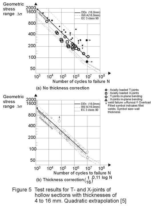
For thicknesses of 4 to 16 mm:
Ds
t = Dst = 16 mm .For thicknesses of 16 mm and more:
Ds
t = Dst = 16 mm .For thicknesses below 4 mm no guidance is given, since the fatigue behaviour may be adversely affected by the welding imperfections at the root of the weld.
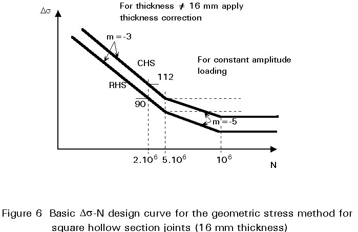
Various investigations have shown that the fatigue limit, i.e. where the Ds-N line changes to a horizontal line, depends on the notch effect. For example, for basic steel, the fatigue limit for constant amplitude loading might be of the order of 2 ´ 106 cycles, whereas for welded connections with high peak stresses it will be about 107 cycles. Many offshore codes and also the IIW recommendations adopt 107 for tubular connections. In Eurocode 3 [1], one general limit of N = 5 ´ 106 is given.
For random or variable amplitude loading with stresses exceeding the Ds, at 5 ´ 106 certain interaction effects may appear with the result that smaller stress ranges can have an influence on the fatigue life. This is incorporated by changing the slope after 5 ´ 106 cycles to m = - 5. The fatigue limit for variable amplitude loading is given for all welded connections including hollow section joints at 108 cycles. In certain offshore codes 2 ´ 108 is given. However, no tests are available to check whether this is correct.
Various re-analyses of test results [5, 8, 9] have shown that for the geometric stress or hot spot stress concept, the following classes (stress range at 2 ´ 106 cycles) can be adopted for hollow section joints with 16 mm thickness:
|
Class (16 mm) |
|
|
Circular hollow section joints Square or rectangular hollow section joints |
112 N/mm2 90 N/mm2 |
For other thicknesses, the thickness corrections according to Equations (5) and (6) have to be adopted for N £ 5 ´ 106. For N > 5 ´ 106 the Ds-N curve remains parallel to the Ds-N line for 16 mm thickness (thus, the same thickness effect is used as for N = 5 ´ 106).
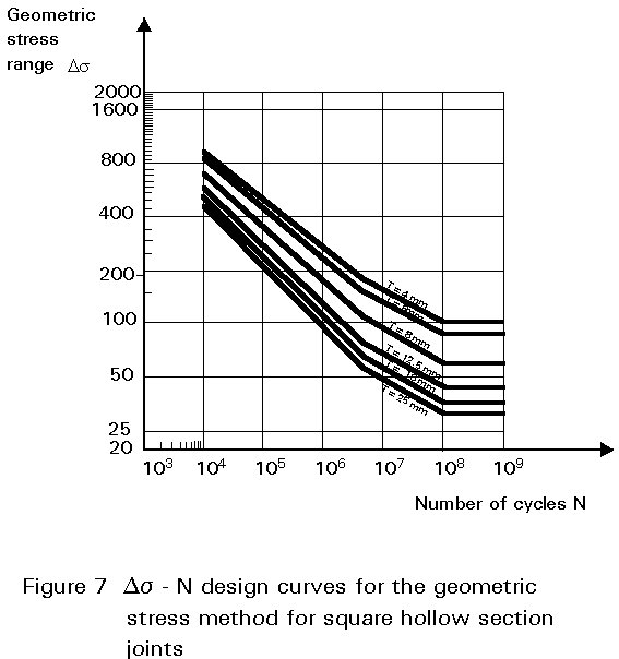
As stated above, the Ds curves for thicknesses of 16 mm and larger have a slope m = -3, whereas below 16 mm the curves change to a smaller slope due to the thickness correction.
Figure 6 shows the resulting basic curves for 16 mm thickness. In Figure 7 this is worked out for square hollow section joints including the thickness correction. ECSC and CIDECT [5, 9] research has proved that for thicknesses up to 8 mm, these curves can be used for butt welded and fillet welded connections or for combinations of both welds. For thicknesses larger than 8 mm, butt welds should be used.
In Eurocode 3 [1], Class 90 is given for butt welded joints with controlled weld profile and lower classes are given for butt welds (Class 71) and fillet welds (Class 36). However, it is stated that higher values may be used if sufficient data is available for justification. The outcome of the research with basic classes of 112 and 90 for 16 mm thickness will be the basis for the next revision of Eurocode 3.
In Eurocode 3, Ds -N curves are given for N = 104 cycles and higher [1]. It is further stated that the stress range should not exceed 1,5 times the yield stress in order to avoid alternating yielding. In general, in the case of low cycle fatigue, the stress range concept is not valid and the fatigue strength is determined more by strain range. This limitation is true for concepts based on nominal stress; but with a geometric stress concept the geometric peak stress ranges are considered, which are only locally present.
As shown in Figure 5, the fatigue test results of hollow section joints for N = 103 are still in line with the Ds-N curves given. However, this basis might result in very high theoretical stress ranges (in some cases 5 times the yield stress). These extended Ds-N curves can be used; but a brittle failure check should be carried out to determine the critical crack depth.
For each potential crack location the long term distribution of relevant stress ranges should be established and the probable fatigue life should satisfy the Palmgren-Miner linear cumulative damage rule: S ni/Ni £ 1,0.
An arbitrary joint could be checked by following the steps given below, also shown in a flow chart in Figure 8, for a T- and X-joint of square hollow sections.
In the previous section it has been shown that the geometric (peak) stress range largely determines the fatigue life. The stress range depends on the type of joint, geometry and loading. If the fatigue strength were to be based on nominal stress ranges, then on the one hand it would be simpler for the designer, but on the other hand, an atlas would be required to cover all cases [10].
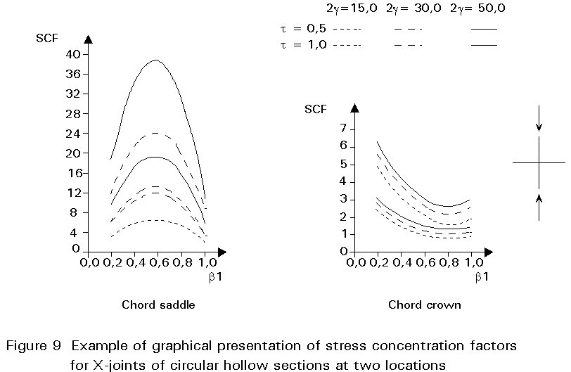
The classification method now offers a compromise between both concepts. The test results are analyzed based on nominal stress range in the brace and then grouped together in such a way that the main influencing geometrical parameters are taken into account. For connections in which the geometrical stress concentration factor varies to a large extent, e.g. X- or T-joints, see Figure 9, such grouping is not possible. However, for K- and N-joints, a classification can be adopted if the thickness parameter to/ti is included and certain parameters are kept nearly constant, e.g. gap, overlap, angle. Further, stringent limitations should be made for the range of validity. This approach is currently included in Eurocode 3 [1] for K and N joints with thicknesses up to 12,5 mm. A more detailed description is given in Lecture 12.4.2.
Other methods [7, 10] are also given in the literature and guides, e.g.
This method, developed at the University of Karlsruhe, is also based on the fact that the stress concentration factor is indirectly taken into account by giving nominal stress ranges at 2 ´ 106 (all classes) in relation to the joint geometry parameters and loading. The data is presented in diagrams. The Ds-N curve to be used is then fixed by the design class. This method is not used at present.
This method has a certain relation with the classification method. However, here the punching shear stress range is taken as the basis instead of the nominal stress range in the brace. This method is used in American codes, such as the API and AWS standards.
In many Japanese publications the stress range is related to the static strength for the same hollow section joints, but with a yield stress fy = 235 N/mm2. As fatigue is a quite different phenomenon from static strength, one could expect poor correlation between the test results and the Ds -N line. However, the correlation is not worse than for the other simplified methods discussed above.
This funding may be explained by the fact that the static strength depends on the same geometrical parameters which influence the geometric stress and also that the incremental load capacity of the joint between initial localized yielding and failure has some relation to the stress gradient. Thus, within certain parameter ranges, a reasonable relationship can be obtained. This method has of course no general validity since various factors are not included, e.g. tension vs compression loading, effect of secondary bending moments, etc.
In lattice girder joints (e.g. K- and N-joints) secondary bending moments exist. For static design these moments are not important if the critical members or joints have sufficient rotation capacity. However, for fatigue design the peak stress range is the governing parameter and secondary bending moments influence the peak stress (range). As a consequence, secondary bending moments have to be considered in fatigue design.
Secondary bending moments are caused by various influences, such as:
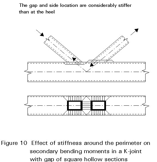
Figure 10 shows, as an example, a K-joint in which three sides at the intersection are stiffer than the side at the heel, resulting in a secondary bending moment since the reaction force is not in line with the force in the brace member.
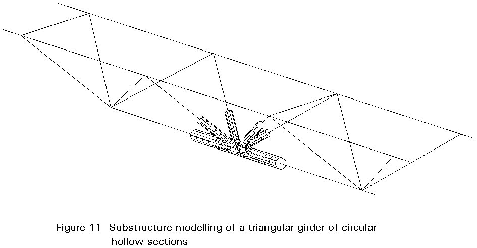
The secondary bending moment can only be accurately taken into account if the joints are modelled as substructures with finite elements as shown in Figure 11. However, such modelling is still the future for engineering offices.
To avoid these complicated analyses, Eurocode 3 [1] gives factors to account for the secondary bending moment effects (Tables 1a and 1b). The stress ranges obtained for axial loading should be multiplied by these factors if the secondary bending moments are not included in the analysis. The values given in these tables are based on measurements in actual girders and tests as well as finite element calculations. Comparison of the various values shows that the secondary bending moments in girders with N-joints are larger than those in girders with K-joints. The secondary bending moments in girders of rectangular or square hollow section joints are larger than those in girders with circular hollow section joints. These effects are caused by the stiffness along the intersection perimeter and the stiffness of the brace members (vertical brace for N-joints). In general, overlap joints of rectangular hollow sections give lower secondary bending moments in the braces than in the case of gap joints. For girders of circular hollow sections a similar effect is given in the tables, although current research does not confirm this [11]. More evidence will be obtained when current research projects are finished.
For simple connections, such as butt welded end-to-end connections or hollow sections connected to plates, a simple classification is used as for other sections. The same procedure is followed for attachments, cover plates, etc. The classification is in line with the classifications given for similar welded details of I-sections, see Lecture 12.4.2.
For hollow section joints, the same partial safety factors apply for the stress range as for other structures loaded in fatigue. Eurocode 3 recommends factors (Table 2) which depend on the type of structure (fail safe and non fail safe) and the possibility of inspection and maintenance. For more detailed information, see Lecture 12.8.
Eurocode 3 has adopted the Palmgren-Miner rule to determine cumulative fatigue damage, i.e.:
D = ![]() (7)
(7)
Although the real damage also depends on the spectrum of the loading and the sequence of stress ranges, the Miner rule is the simplest available for determining damage. Its use gives results which are not worse than those given by other rules. For more detailed information, see Lecture 12.2.
[1] Eurocode 3: "Design of Steel Structures": ENV 1993-1-1: Part 1, General Rules and Rules for Buildings, CEN, 1992.
[2] Steel in marine structures, Proceedings of the 2nd International ECCS Offshore Conference, Institut de Recherches de la Siderurgie Française, Paris, October 1981.
[3] Gurney, T.R.: "Fatigue of welded structures", Cambridge, 2nd ed.
[4] Van Delft, D.R.V.: "A two dimensional analysis of the stresses at the vicinity of the weld toes of welded tubular joints", 1981, Report 6-81-8, Stevin Laboratory, Delft University of Technology.
[5] Van Wingerde, A.M.: "The fatigue behaviour of T- and X-joints made of square hollow sections", Ph.D. thesis, Delft University of Technology, 1992.
[6] Noordhoek, C. and De Back, J., Eds.: Steel in Marine Structures, Proceedings of the 3rd International ECSC Offshore Conference on Steel in Marine Structures (SIMS '87), Delft, The Netherlands, June 15-18, 1987.
[7] Marshall, P.W.: "Design of welded tubular connections: Basis and use of AWS code provisions", Ph.D. thesis, Elsevier Applied Science Publishers Ltd., Amsterdam/London/New York/Tokio.
[8] Reynolds, A.G., Sharp J.V.: "The fatigue performance of tubular joints - An overview of recent work to revise Department of Energy guidance", 4th International Symposium of Integrity of Offshore Structures, p. 261-277, Elsevier Applied Science Publishers Ltd., Amsterdam/ London/New York/Tokio. Glasgow, U.K., July 1990.
[9] Wardenier, J., Mang, F., Dutta D.: "Fatigue strength of welded unstiffened RHS joints in lattice structures and Vierendeel girders". ECSC Final Report, ECSC 7210-SA/111.
[10] Wardenier, J.: "Hollow Section Joints", Delft University Press, 1982, ISBN 90.6275.084.2.
[11] Romeijn, A., Wardenier, J., de Komming, C. H. M., Puthli, R. S,, Dutta,D.: "Fatigue Behaviour and Influence of Repair on Multiplanar K-Joints Made of Circular Hollow Sections". Proceedings ISOPE '93, Singapore.
|
Table 1a Coefficients to account for secondary bending moments in joints of lattice girders made from circular hollow sections |
||||
|
Type of joint |
Chords |
Verticals |
Diagonals |
|
|
Gap joints |
K |
1,5 |
- |
1,3 |
|
N |
1,5 |
1,8 |
1,4 |
|
|
Overlap joints |
K |
1,5 |
- |
1,2 |
|
N |
1,5 |
1,65 |
1,25 |
|
|
Table 1b Coefficients to account for secondary bending moments in joints of lattice girders made from rectangular hollow sections |
||||
|
Type of joint |
Chords |
Verticals |
Diagonals |
|
|
Gap joints |
K |
1,5 |
- |
1,5 |
|
N |
1,5 |
2,2 |
1,6 |
|
|
Overlap joints |
K |
1,5 |
- |
1,3 |
|
N |
1,5 |
2,0 |
1,4 |
|
Table 2 Partial safety factors gM according to Eurocode 3
|
Inspection and access |
"Fail safe" structures |
Non "fail safe" structures |
|
Periodic inspection and maintenance. Accessible joint detail. |
g M = 1,00 |
g M = 1,25 |
|
Periodic inspection and maintenance. Poor accessibility. |
g M = 1,15 |
g M = 1,35 |