ESDEP WG 10
COMPOSITE CONSTRUCTION
To describe the behaviour of composite columns and to explain the design method for uniaxial and biaxial bending, including the determination of internal moments and forces.
Lecture 7.2: Cross-Section Classification
Lecture 7.3: Local Buckling
Lecture 7.10: Beam Columns
Lecture 10.2: Behaviour of Beams
Lecture 10.8.1: Composite Columns I
Lecture 10.6.1: Shear Connection I
This lecture shows how the plastic resistance of a composite column, under combined compression and bending, can be calculated. The design method given in Eurocode 4 for uniaxial and biaxial bending is explained [1]. Simplified methods for determining second order internal moments are also given. The influence of shear force on the moment resistance is considered.
Lecture 10.8.1, on composite columns, explained the simplified method for designing columns subject to axial compression only and outlined the restrictions on its application. The rules regarding local buckling, creep and shrinkage of concrete were also described.
This lecture assumes knowledge of the above and describes the design of columns subject to combined compression and bending, and columns subject to shear.
The design for compression and bending is carried out in stages, as follows: the composite column is examined, isolated from the system; in so doing, the end moments which result from the analysis of the system as a whole (including second order effects) are taken to act on the individual element; internal moments and forces within the column length are determined from the end moments, the normal forces and any transverse forces; for slender columns second order effects are included. In the simplified method of Eurocode 4 [1] imperfections within the column length need not be considered as they are taken into account in the determination of the column resistance.
The resistance of the column to compression and bending is determined with the help of a cross-section interaction curve. This curve may also be used to assess the influence of shear forces on the column.
The influence of second order effects may be neglected in the analysis of bending moments for braced and non-sway systems, provided that:
£ 0,2 (2 - r) (1)
where r is the ratio of the smaller to the larger end moment (see Figure 1).
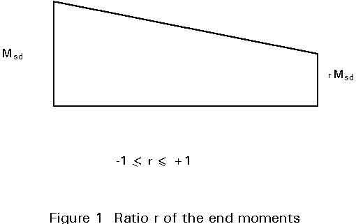
For transverse loading within the column length r = 1.
The flexural stiffness, which is necessary for the analysis of second order effects, can be calculated by multiplying the maximum first order bending moment by a factor k:
 (2)
(2)
where
NSd is the design normal force.
Ncr is the critical load (see Lecture 10.8.1, Equation (10) with le as the length of the column.
b
is the moment factor.For columns with transverse loading within the column length the value for ß must be taken as 1,0. For pure end moments, ß can be determined from:
b
= 0,66 + 0,44r but b ³ 0,44 (3)Figure 2 shows how the cross-section of a composite column can be checked, by means of the interaction curve M-N. First the resistance of the column under axial compression is determined according to the previous lecture. This resistance is defined by the reduction factor c (Lecture 10.8.1, Equation 16). For the factor c, a value for the moment mk representing the moment due to imperfection, can be read off the interaction curve.
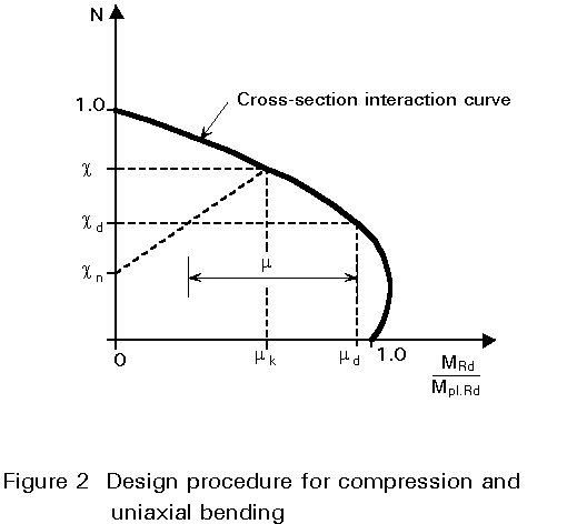
The influence of this moment is assumed to decrease linearly to the value cn. For a normal force of cd = NSd / Npl.Rd the moment factor m represents the remaining moment resistance. It must be shown that:
MSd £ 0,9 m Mpl.Rd (4)
In certain regions of the interaction curve, the normal force increases the moment resistance (m > 1,0). If bending moment and normal force are independent of each other, the value of m must be limited to 1,0. The value cn accounts for the fact that imperfection and bending moment do not always act together unfavourably.
For end moments, cn may be calculated as:
cn = ![]() (5)
(5)
with r is the ratio of end moments according to Figure 1.
If transverse loads occur within the column length, then cn must be taken as zero, i.e. r = 1.
The reduction of the resistance moment, in Equation (4), by 10% accounts for the simplifications that have been made. The interaction curve has been determined without considering the strain limitations in the concrete. Hence the moments, including second order effects, Equation (2), may be calculated using the effective flexural stiffness (EI)e based on the complete concrete area of the cross-section.
The interaction curve described in the Section 4, can be found by adjusting the neutral axis across the whole cross-section and determining the internal moments and forces from the resulting stress blocks. This can only be done adequately by a computer program, due to the number of equations to be solved. It is, however, possible to calculate certain points on the interaction curve quite simply without the help of a computer. These points (A-E) are marked on the interaction diagram in Figure 3, and are connected by a series of straight lines. These lines are sufficiently exact for most design purposes.
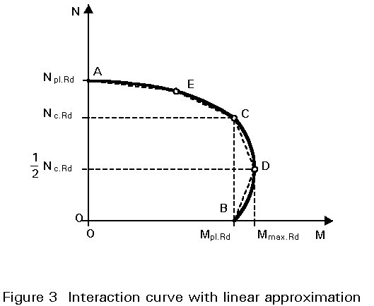
Figure 4 shows the stress distributions at each point, A, B, C, D and E for the example of a concrete filled rectangular hollow section.
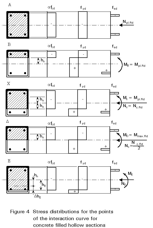
Point A marks the resistance to normal force:
NA = Npl.Rd (6)
MA = 0 (7)
Point B shows the stress distribution for moment resistance only:
NB = 0 (8)
MB = Mpl.Rd (9)
Here it can be seen, that in the determination of the resistance of the cross-section, concrete regions in tension are taken as being cracked and ineffective.
The moment of resistance at point C is identical to that at point B, since the stress resultants from the additionally compressed parts nullify each other in the central region of the section.
These additionally compressed regions, however, create an internal normal force which is equal to the plastic axial resistance of the concrete member alone. This can be understood by adding up the stress distributions of point B and C; the normal force balance does not change since there is no resulting normal force for point B. All steel parts compensate each other and the compression area of the concrete at point B is identical with the concrete tension area of point C. The axial force is, therefore, given by the following expression:
NC = Nc.Rd = Ac a fcd (10)
where
a
is 1,0 for concrete filled profilesfcd is the design strength of the concrete
MC = Mpl.Rd (11)
At point D, the plastic neutral axis coincides with the centroidal axis of the cross- section, and the resulting normal force is half of the resistant force at C. This stress distribution allows rapid and simple calculation of the moment and normal force.
ND = Nc.Rd / 2 (12)
MD = Mmax.Rd (13)
Mmax.Rd = Wpa fyd + 0,5 Wpc a fcd + Wps fsd (14)
where
Wpa, Wpc and Wps are the plastic moments of resistance of the structural steel, concrete and reinforcement.
fyd, fcd and fsd are the respective design strengths of the materials.
For point E, the neutral axis is placed between that of point C and the edge of the cross-section in such a way that the stress resultant can easily be calculated. Point E need not be determined in all cases.
The positions of the neutral axis for point B (Mpl.Rd), and similarly point C, i.e. the distance hn, can be determined from the difference in stresses at point C and point B (see Figure 5). Since parts are generally of a rectangular shape in the central region the cross-section, the resulting forces dependent on hn can easily be determined. The sum of these forces is equal to Nc.RD, as shown above. This calculation enables the equation defining hn to be determined. This equation is different for various types of sections.
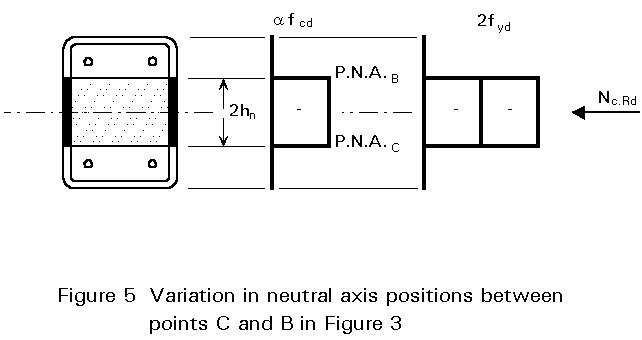
For the example of the concrete filled rectangular hollow section:
hn = ![]() (15)
(15)
The moment resistance Mpl.Rd can be simply calculated from the difference of stresses between point D and point B (Figure 6).
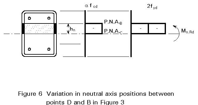
Mn.Rd = wpan fyd + 0,5 Wpcn a fcd + Wpsn fsd (16)
where
Wpan, Wpcn and Wpsn are the plastic moments of resistance of the areas in the region of 2 hn
For the moment resistance Mpl.Rd:
Mpl.Rd = Mmax.Rd - Mn.Rd (17)
For concrete encased I-profiles and for concrete filled tubes, the respective formulae are given in Annex C of Eurocode 4 [1].
The advantage of this method of calculation is its applicability to any doubly-symmetrical cross-section. Even for more complex sections (e.g. Lecture 10.8.1, Figure 1c or (f) the characteristic points on the interaction diagram can easily be determined.
The linear interaction diagram ABCD can sometimes underestimate the value of the moment due to the imperfection mR.
If, for example, the deviation between the polygonal path and the exact curve is very large in the region of the imperfection moment, at the height of c in Figure 2, and small at the normal force cd, the imperfection taken into account is too small. In this case point E is nearly midway between point A and point C and has to be determined.
For concrete encased I-sections, with bending about the strong axis of the steel section, the exact interaction curve is almost linear between point A and C, so that point E need not be determined in this case.
For the design of a column under compression and biaxial bending the load resistance for each axis has to be evaluated separately. It will then be clear which of the axes is more likely to fail. The imperfection then needs to be considered for this direction only (see Figure 7).
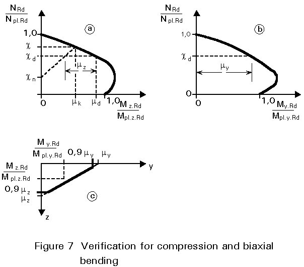
The combined bending must also be checked using the relative values of moment resistance my and mz, and a new interaction curve (see Figure 7c). This linear interaction curve is cut off at 0,9 my and 0,9mz; the existing moments My.Sd and Mz.Sd, related to the respective resistance, must lie within the new interaction curve. The following equations result:
My.Sd/(myMply.Rd) - Mz.Sd/(mzMplz.Rd) £ 1,0 (18)
and
My.Sd/(my Mply.Rd) £ 0,9 (19)
Mz.Sd/(mz Mplz.Rd) £ 0,9 (20)
Bond stresses between the steel profile and the concrete must not exceed the following values:
- for the flanges 0,2 N/mm2
- for the webs 0,0 N/mm2
An exact determination of the bond stresses between structural steel and concrete is difficult. Stresses in the composite section may be determined in a simplified way, using elastic theory, or by means of the plastic resistance of the cross-section. The variation of stresses in the concrete member, between two critical sections, can be used for the determination of bond stresses.
In a similar way division of the shear force between structural steel and concrete can be made. The shear force to be resisted by the concrete must be considered according to Eurocode 2 [2], whereas the shear force to be resisted by the steel section can be checked, if necessary, by using an interaction relationship. Figure 8 shows the reduction of normal stresses in the areas which transfer shear stresses.
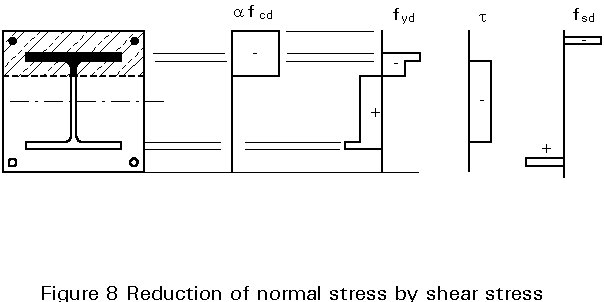
This reduction of the yield limit, in the parts which transfer shear, can be transformed, for the purposes of design, into a reduction of the member thickness. The influence need not be considered if:
Va.Sd < 0,5 Vpl.a.Rd (21)
where
Va.Sd is the part of the design shear resisted by the steel section
Vpl.a.Rd is the resistance of the steel cross-section in shear
Vpl.a.Rd = Av ![]() (22)
(22)
where
AV is the shear area of the structural steel cross-section.
The reduction in shear area is given by:
 (23)
(23)
For a concrete encased I-section, with bending about the strong axis:
red AV = red tw h (24)
Using this reduced thickness, red tw, the method given in Section 5, for the determination of the cross-section interaction curve, can be applied without any modification.
For simplicity, division of the shear force between the steel cross-section and the concrete is often neglected. For concrete filled hollow profiles, for example, the total shear force is typically allotted to the steel section alone.
Where loads are introduced into a composite column, it must be ensured that within a specified introduction length, the individual components of the cross-section are loaded according to their resistance. For this purpose, in a manner similar to Section 7, a division of the loads between steel and concrete must be made.
In order to estimate the exact distribution of the load to be introduced, the stress distributions at the beginning and end of the region of introduction must be known. From the differences in these stresses the loads to be transferred to the cross-section components may be determined. The length II of the region of load introduction should not exceed the value:
II £ 2 d (25)
where d is the cross-section dimension normal to the bending axis.
The loads can be simply distributed using the plastic resistances:
 (26)
(26)
![]() (27)
(27)
![]() (28)
(28)
![]() (29)
(29)
where
Na.Rd is the normal force resistance of the structural steel section.
Ncs.Rd is the normal force resistance of the reinforced concrete section.
Npl.Rd is the normal force resistance of the total composite cross-section.
Ma.Rd is the moment resistance of the structural steel section.
Mcs.Rd is the moment resistance of the reinforced concrete section.
Mpl.Rd is the moment resistance of the total composite cross-section.
For the determination of Mcs.Rd the calculation should be based on Section 5, neglecting the steel section.
If loads are first introduced through a connection to the steel, the elements of load introduction, e.g. headed studs, must be designed to transmit the concrete components of the loading, Ncs.Sd and Mcs.Sd. In the case of load introduction from the concrete into the steel member, e.g. through brackets, the respective steel forces and moments, Na.Sd and Ma.Sd, must be taken as the basis for design.
For single-storey columns, head plates are generally used as the elements for load introduction. Special detailing is necessary for continuous columns. For these cases headed studs have proved to be economic when used with open cross-sections (see Figure 9). The forces on the outward stud connectors are transmitted to the flanges and the following friction force results:
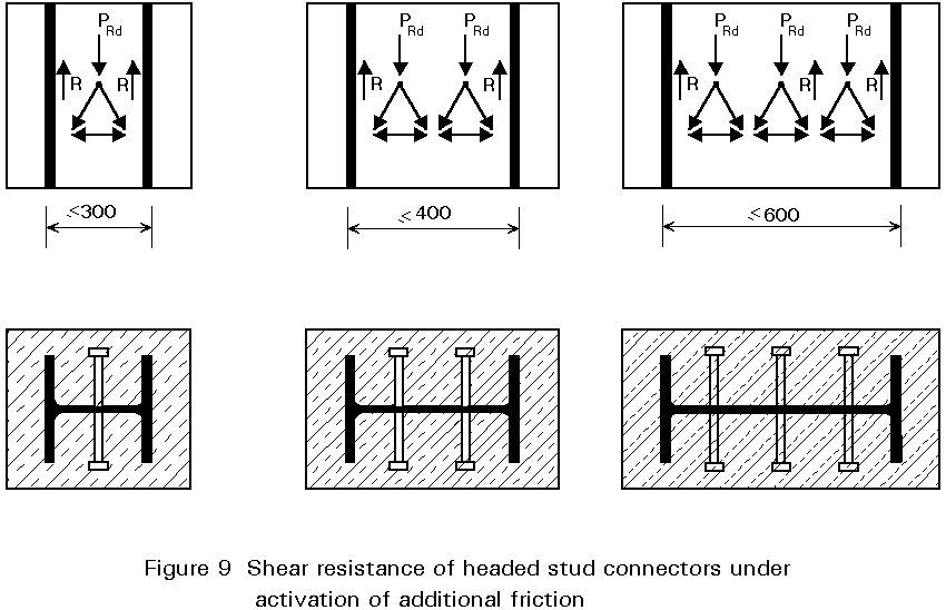
R = m PRd / 2 with m = 0,5 (30)
where PRd is the design resistance of one headed stud connector.
For introducing forces into continuous concrete filled hollow profiles, the use of gusset plates, punched through the profile, is a very economic solution. Due to the effect of confinement, high normal stresses can occur beneath the edge of the gusset (Figure 10).
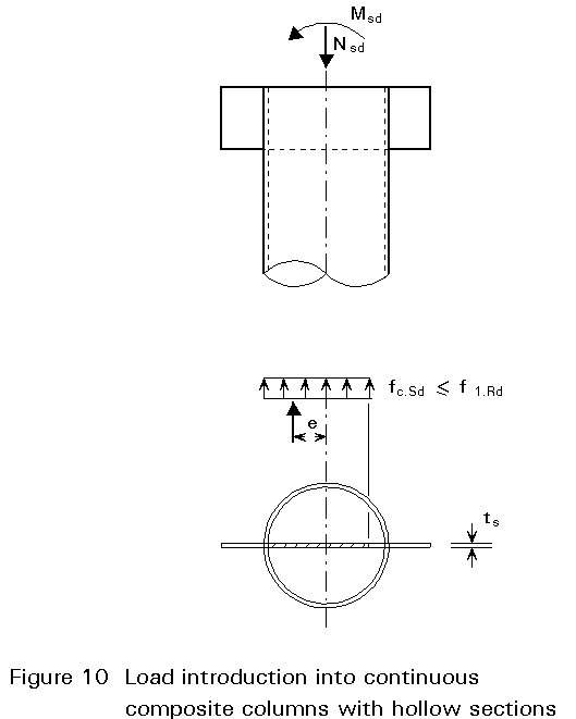
f1.Rd = (0,6 fck + 35,0)(1/gc)Ö(A/A1) (31)
f1.Rd £ Nc.Rd/A1 (32)
where
A is the total area of the concrete core.
A1 is the area beneath the edge of the gusset.
Equation (31) is taken from tests and has not yet been statistically verified.
[1] Eurocode 4: "Design of Composite Steel and Concrete Structures: ENV1994-1-1: Part 1.1: General rules and rules for building, CEN, (in press)
[2] Eurocode 2: "Design of Concrete Structures: ENV 1992-1-1: Part 1.1: General rules and rules for building, CEN, 1992.