ESDEP WG 7
ELEMENTS
To explain the use of the European buckling curves and to introduce the concept of torsional and flexural-torsional buckling.
Lecture 6.1: Concepts of Stable and Unstable Elastic Equilibrium
Lecture 6.6.1: Buckling of Real Structural Elements I
Lecture 7.5.1: Columns I
Lecture 7.2: Cross-Section Classification
Lecture 7.10.1: Beam Columns I
Worked Example 7.5: Column Design
The analysis of imperfections, leading to the derivation of the Ayrton-Perry formula and the European buckling curves, is explained and justified. The concepts of torsional and flexural-torsional buckling are introduced for the case of simple compression members.
The behaviour of real steel structures is always different from that predicted theoretically; the main reasons for this discrepancy are:
Of the above, some are important in the buckling of slender columns (geometrical imperfections), others in the compression of stub columns (material inelasticity) and others in the buckling of columns of medium slenderness (geometric imperfections and residual stresses). The behaviour of these three types of columns is described in Lecture 7.5.1.
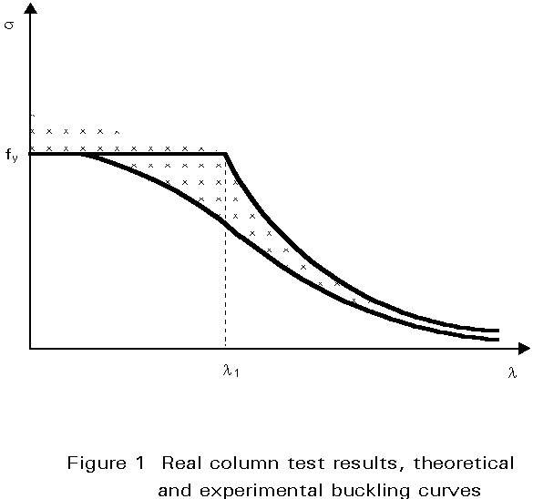
In reality, all the imperfections act together simultaneously and their effect depends on their individual intensity and on the slenderness of the column. An experimental study of many columns with various characteristics gives the results shown in Figure 1. The results of the tests should be below the Euler buckling curve because initial out-of-straightness, eccentricity of applied loads and residual stresses all decrease the allowable buckling load; for small slenderness (stub columns), however, it is possible to find some results above the yield stress line because of possible strain-hardening. A safety curve obtained through a statistical analysis is always situated under the minimum experimental values and has the form shown in Figure 1; the plateau is necessary to limit the allowable stress to the yield value. This is the general form of the European buckling curves [1, 2].
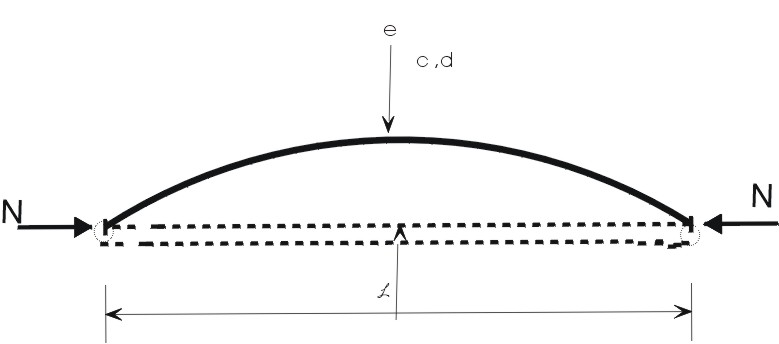
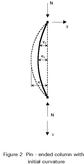
Assuming that the initial deflection of a pin-ended column of length l, has a half sine-wave form with magnitude eo (Figure 2), the initial deformation along the column can be written as:
![]() (1)
(1)
The differential equation for the deformation of such a pin-ended column loaded by an axial force N is:
![]() (2)
(2)
Combining this with the expression for yo, and taking into account the boundary conditions, the solution of this equation is:
![]() (3)
(3)
The maximum total deflection, e, of the column is then:
![]() (4)
(4)
and the ratio 1/(1 - N/Ncr) is generally called the "amplification factor".
Taking into account the maximum bending moment, Ne, due to buckling, the equilibrium of the column requires that:
![]() (5)
(5)
where fy is the yield stress.
If N is the maximum axial load, limited by buckling, and sb the maximum normal stress (sb = N/A), this becomes:
![]() (6)
(6)
or, introducing scr, the Euler critical stress (scr = p2E/l2) and including the value of e:
![]() (7)
(7)
which can be written as:
(scr - sb) (fy - sb) = sb scr eo A/W (8)
This equation is the basic form of the Ayrton-Perry formula.
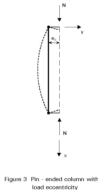
If the axial compression load is applied with an eccentricity ec on an initially straight pin-ended column (Figure 3), a bending moment (N ec) is introduced which increases the buckling effect. This effect obviously increases along with axial load.
It is possible to show that the total maximum deflection e of the column is equal to:
e = ec - ec/{cos[l/2 (N/EI)1/2]} (9)
and the "amplification factor" to: 1/cos [p/2 (N/Ncr)1/2]
Now, if the combined effect of the initial deflection and of the eccentricity of loading is considered, the stress is approximately equal to:
![]() (10)
(10)
This relationship is correct within a few percent for all values of sb from 0 to scr.
The classical form of the Ayrton-Perry formula is:
(scr - sb) (fy - sb) = h scr sb (11)
This is the form of Equation (8) if h = (eo A) / W
The coefficient h represents the initial out-of-straightness imperfection of the column but it can also include other defects such as residual stresses in which case it is called the "generalized imperfection factor".
It is possible to write the Ayrton-Perry formula under another form:
(scr / fy - ![]() ) ( 1 -
) ( 1 -
![]() ) = h
) = h
![]() scr / fy
(12)
scr / fy
(12)
where: ![]() = sb / fy
= sb / fy
If ![]() 2 = fy / scr then, dividing by scr / fy, gives:
2 = fy / scr then, dividing by scr / fy, gives:
(1 - ![]()
![]() 2) (1 -
2) (1 -
![]() ) = h
) = h![]() (13)
(13)
or: ![]() 2
2![]() 2 -
2 -
![]() (
(![]() 2 + h + 1) + 1 = 0
(14)
2 + h + 1) + 1 = 0
(14)
This form leads to the European formulation [1].
The generalized imperfection factor takes into account all the relevant defects in a real column when considering buckling: geometric imperfections, eccentricity of applied loads and residual stresses; inelastic properties are not considered because they only influence stub columns. The generalized imperfection factor can be expressed through the coefficient h representing the effect of deflections:
![]() (15)
(15)
where g = l / eo, represents the equivalent geometrical imperfection (which is the ratio of the length over the equivalent initial curvature of the column).
Then using L = l.i, W = I / v and i2 = I / A, h can be written as:
h = l / g (i/v) (16)
where (i/v) is the relative diameter of the inertia ellipse in the axis where buckling occurs.
As l =![]() h (E/fy)1/2, introducing the plateau
h (E/fy)1/2, introducing the plateau
![]() = 1 when
= 1 when
![]() £
£ ![]() o, the previous relationship can be written as:
o, the previous relationship can be written as:
![]() (17)
(17)
because all the European buckling curves were established with fy = 255 MPa (the real value of the yield stress having a very small influence).
Using h expressed as:
h
= a(the smallest solution of the Equation (14) is:
![]() = {1 + a(
= {1 + a(![]() -
-
![]() o)
+
o)
+ ![]() 2
- [1 + a (
2
- [1 + a (![]() -
-
![]() o)+
o)+
![]() 2]2
- 4
2]2
- 4![]() 2}1/2
/ 2
2}1/2
/ 2![]() 2
(19)
2
(19)
Multiplying by the conjugated term and choosing ![]() o = 0,2, this relationship gives the European formulation:
o = 0,2, this relationship gives the European formulation:
c = 1 / {f
+ [f2 -where:
f
= 0,5 [1 + a (c
is the reduction factor considered in Eurocode 3 [1].The different shapes of cross-sections used to design steel columns have the coefficient a varying from 0,21 to 0,76 and it is possible to represent the real behaviour of all classical columns using the four curves (a, b, c and d) shown in Figure 4, a increasing with the imperfections.
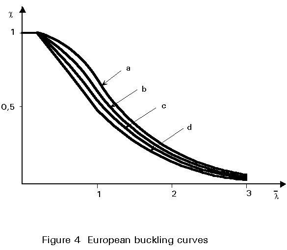
a
takes into account two kinds of imperfections (geometrical and mechanical). It can be written as a = a1 + a2, where a1 represents the mechanical and a2 the geometrical imperfections. Considering only the geometrical imperfections, the European buckling curves were established with an initial curvature equal to L/1000 (Lecture 7.5.1); this givesa2 = 90,15/[1000 (i/v)].
Considering now the equivalent initial deflection: eo = L/g , linked to the generalized imperfection factor h (Equation (15)) and using Equation (18), gives:
eo = a(![]() - 0,2) W / A
(22)
- 0,2) W / A
(22)
which represents the equivalent initial bow imperfection of a pin-ended column including the initial crookedness and the effect of residual stresses; this has to be taken into account in a second order analysis. The design values relative to each European buckling curve are given in Table 1.
For hot-rolled steel members, with the type of cross-sections commonly used for compression members, the relevant buckling mode is generally flexural buckling; however, in some cases, torsional or flexural-torsional modes may govern and these must be investigated for all sections with small torsional resistance.
Concentrically loaded columns can buckle by flexure about one of the principal axes (classical buckling), twisting about the shear centre (torsional bucking) or a combination of both flexural and twisting (flexural-torsional buckling).
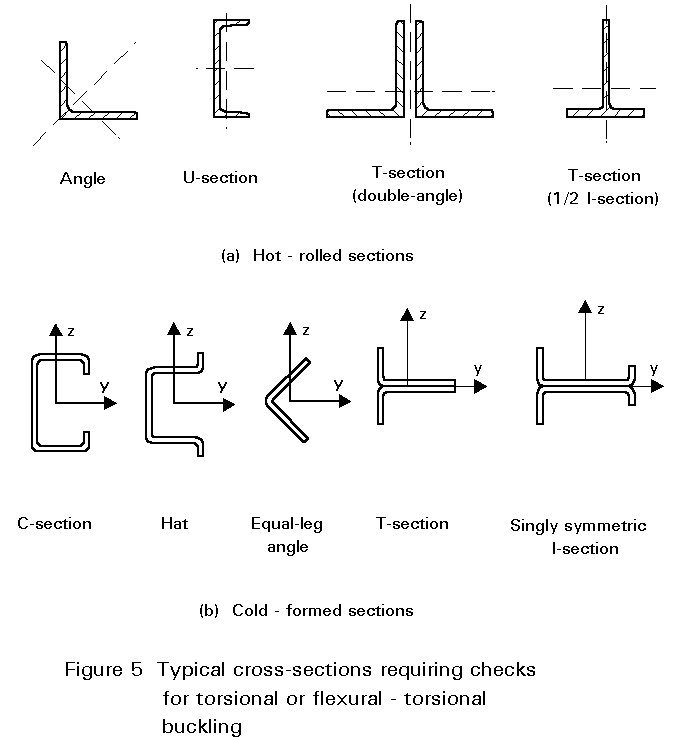
Torsional buckling can only occur if the shear centre and centroid coincide and the cross-section can rotate; this leads to a twisting of the member. Z-sections and I-sections with broad flanges can be subject to torsional buckling; pylons, fabricated from angle sections, must also be checked for this kind of instability.
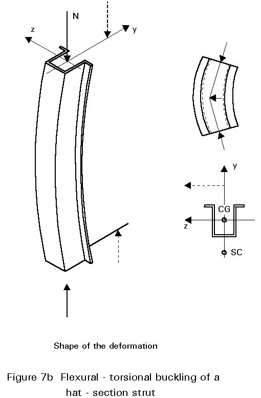
Symmetrical sections with axial load not in the plane of symmetry, and non-symmetrical sections such as C-sections, hats, equal-leg angles, T-sections and singly symmetrical I-sections, i.e. sections where the shear centre and the centroid do not coincide, must be checked for flexural-torsional buckling.
Figure 5 gives examples of sections which must be checked for torsional or flexural-torsional buckling.
The analysis of torsional bucking is quite complex and is too long to be included here. The critical stress depends on the boundary conditions and it is very important to evaluate precisely the possibilities of rotation at the ends. The critical stress depends on the torsional stiffness of the member and on the resistance to warping deformations provided by the member itself and by the restraints at its ends.
The differential equation for torsional buckling is:
![]() (23)
(23)
and the critical load for pure torsional buckling, Ncrq , is:
![]() (24)
(24)
where ro is the polar radius of gyration, G the shear modulus of elasticity, N the axial load, q the twist angle, ID the torsion constant, and Iw the warping constant. Lecture 7.9.2 gives more details about the physical meaning and the computation of the warping constant.
To check a compression member with torsional buckling, a new reference slenderness
![]() must be evaluated:
must be evaluated:
![]() =
Ö(fy/scrq)
(25)
=
Ö(fy/scrq)
(25)
where scrq is the elastic critical stress for torsional buckling obtained with the critical load Ncrq (Equation (24)).
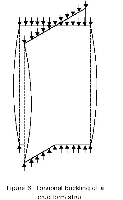
Generally flexural buckling occurs at a lower critical stress than torsional buckling.
Figure 6 illustrates this phenomenon for the case of a cruciform strut.
This is the combination of flexural and torsional buckling and its analysis is too complex to be covered in detail here.
The three basic equilibrium equations governing this sort of buckling are:
![]() (26)
(26)
![]() (27)
(27)
![]() (28)
(28)
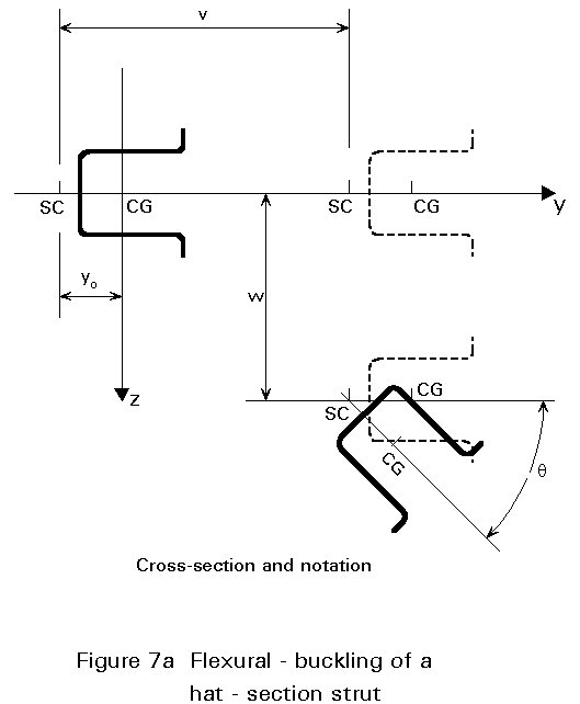
where, yo and zo are the coordinates of the shear centre and v and w are the deflections, as shown in Figure 7.
The critical load for pure torsional buckling is obtained from the lowest root of the following equation:
ro2 (Ncr - Ncrz) (Ncr - Ncry) (Ncr - Ncrq ) - ...
... Ncr2 zo2 (Ncr - Ncry) - Ncr2 yo2 (Ncr - Ncrz) = 0 (29)
where, Ncry and Ncrz are respectively the critical loads for pure flexural buckling about the axes y and z, and Ncrq is defined by Equation (24).
Cross-sections with one (or two) axis of symmetry give yo (or zo) = 0 leading to a simplification of the previous equation; for example, a section with two axes of symmetry gives:
(Ncr - Ncrz) (Ncr - Ncry) (Ncr - Ncrq ) = 0 (30)
and the members buckle at the lowest of the critical loads without interaction of modes.
This lecture only considered the effects of imperfections on the behaviour of compressed steel columns and, therefore, no end moments are considered. The flexural-torsional buckling, in this case, will be due to the effects such as eccentricity of loading or cross-sectional defects.
To check a compression member with flexural-torsional buckling, a new reference slenderness
![]() must be evaluated in a similar way as for torsional buckling (Equation (25)).
must be evaluated in a similar way as for torsional buckling (Equation (25)).
In this case scrq is the elastic stress for flexural buckling obtained with the critical load relative to flexural-torsional buckling.
[1] Eurocode 3: "Design of Steel Structures": ENV 1993-1-1: Part 1.1: General rules and rules for buildings, CEN, 1992.
2nd Edition, McGraw-Hill, 1961.
Table 1 Design values of equivalent initial bow imperfection eo,d
(from Figure 5.5.1, Eurocode 3) [1]
|
|
||||||
|
Cross-section |
Method of global analysis |
|||||
|
Method used to verify resistance |
Section type and axis |
Elastic, or Rigid - Plastic, or Elastic - Perfectly Plastic |
Elasto-Plastic (plastic zone method) |
|||
|
Elastic [5.4.8.2] |
Any |
a( |
- |
|||
|
Linear [5.4.8.1(12)] |
Any |
a( |
- |
|||
|
Plastic [5.4.8.1(1) to (11)] |
I-section yy-axis |
1,33a( |
a( |
|||
|
I-section zz-axis |
2,0 kg eeff/e |
kg eeff/e |
||||
|
Rectangular hollow section |
1,33a( |
a( |
||||
|
Circular hollow section |
1,5 kg eeff/e |
kg eeff/e |
||||
|
kg = (1 - kd) + 2 kd |
||||||
|
Buckling curve |
a |
eeff |
kd |
|||
|
gM1 =1,05 |
gM1 =1,10 |
gM1 =1,15 |
gM1 =1,20 |
|||
|
a |
0,21 |
l/600 |
0,12 |
0,23 |
0,33 |
0,42 |
|
b |
0,34 |
l/380 |
0,08 |
0,15 |
0,22 |
0,28 |
|
c |
0,49 |
l/270 |
0,06 |
0,11 |
0,16 |
0,20 |
|
d |
0,76 |
l/180 |
0,04 |
0,08 |
0,11 |
0,14 |
|
Non-uniform members: Use value of Wel/A or Wpl/A at centre of buckling length l |
||||||