ESDEP WG 7
ELEMENTS
To explain the application and behaviour of cables.
Lecture 7.4.1: Tension Members I
Lecture 14.4: Crane Runway Girders
Lecture 14.6: Special Single-Storey Structures
Lecture 15B.12: Introduction to Bridge Construction
Lecture 16.2: Transformation and Repair
Worked Example 7.4: Tension Members II
Cable structures (that is those in which the principal element is a cable which transmits only tensile forces) have many and varied applications. This lecture explains how the cables themselves are made and derives the design equations used which take into account their non-linear behaviour.
The use of cables, as tension members, has been on the increase over the last few decades. These cables are composed of high strength steel wires which are bundled together in order to obtain the required tensile resistances. Cable structures provide most interesting and spectacular solutions to modern architectural and engineering problems; they are used in structures such as roofs, hangars, cranes, guyed masts, suspension bridges, cable stayed bridges, transmission towers and ski-lift facilities (see Slides). Compared to conventional structures these require careful consideration as follows:
A cable is a highly flexible member that is primarily capable of transmitting axial forces. It is composed of high strength steel wires which are bundled together; the hierarchy of elements is as follows:
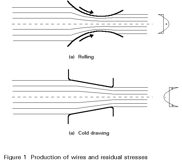
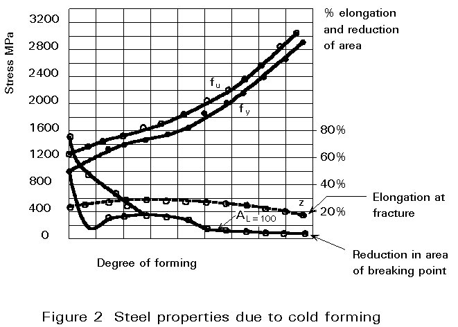
WIRE: This is produced from high-strength steel bars by rolling or cold drawing (Figure 1) thereby reducing the initial area. The cold-forming process results in an increase in the tensile and yield stress and a decrease in the ductility of the steel (Figure 2); it also effects the residual stresses through the wire thickness (Figure 1) since the velocity of the steel running through the area reducing device is different: for cold drawn wires the velocity in the core is larger than at the surface; for rolled wires the opposite is the case.
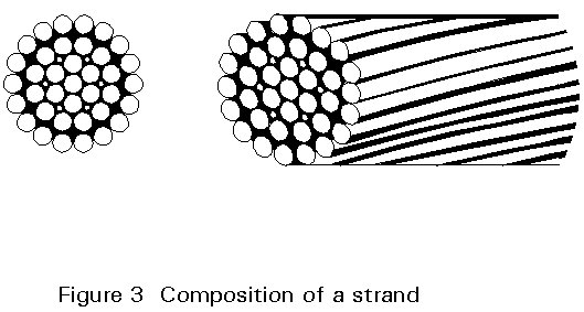
STRAND: This is produced from a series of wires that are normally wound together in a helical fashion (Figure 3).
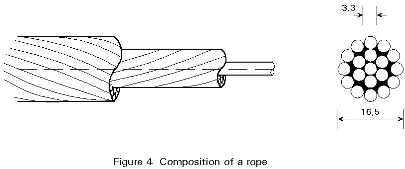
ROPE: This is produced from a series of strands that are also wound together in a helical fashion. If the winding orientation of the strands is, for example, to the left then the strands that produce the rope should be wound together to the right in order to avoid twist of the rope when it is subjected to axial forces (Figure 4).
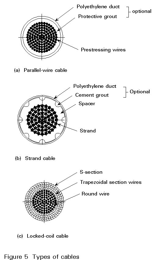
CABLE: Using the elements mentioned above, it is possible to produce cables; the more usual types of cables are:
Due to their chemical composition, and the cold forming process, the tensile strength of the wires is high; it is also normally inversely proportional to the wire diameter. The usual tensile strength is about 1600-1800 N/mm2.
The s -e diagram for this steel has no yield plateau and so the yield strength is conventionally defined as the stress at which the plastic deformation is 0,2%. The value of this strength typically varies between 80 to 90% of the tensile strength.
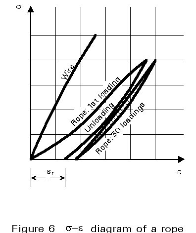
The modulus of elasticity of the strands, ropes and cables is smaller than that of the steel material (wire) of which they are composed (Figure 6). After unloading there is a residual deformation which is not due to plasticity but due to the winding and transportation process, and which stabilises after several loading cycles; this is the reason why, in real structures the cables are post-tensioned after a certain period; after this has been done the modulus of elasticity has a larger value than the initial one.
Mean values of this modulus are normally as follows:
For parallel wire cables E = 200 N/mm2
For locked-coil cables E = 160 N/mm2
For strand cables E = 150 N/mm2
The coefficient of linear thermal expansion has the value of a = 1,2 x 10⁻⁵ per degree centrigrade.
The metallic area of a rope is equal to:
![]() (1)
(1)
where d is the diameter of the rope, and f is a coefficient equal to:
f = 0,55 for multiple strand ropes
f = 0,75 - 0,77 for open spiral ropes
f = 0,81 - 0,86 for locked coil ropes.
The tensile resistance of a rope is equal to:
F = ks Am . fu (2)
where
Am is the metallic area
fu is the tensile strength of the wires
ks is a coefficient equal to:
ks = 0,76 - 0,85 for multiple strand ropes
ks = 0,82 - 0,90 for open spiral ropes
ks = 0,87 - 0,92 for locked coil ropes
ks = 0,93 - 1,0 for parallel wire ropes
The tensile resistance of a complete rope including the anchoring device is equal to:
Fu = ka . ks . Am . fu (3)
where the coefficient ka has values between 0,80 and 1,0 depending on the anchorage system.
The design tensile resistance is then given by the expression:
FRd = Fu /gM (4)
where gM is the partial safety factor.
The design value of the modulus of elasticity is dependent on the stress state under consideration. The s-e diagram of a rope, as presented in Figure 7, is non-linear for the first loading; the rope is subsequently subjected to repeated loading cycles, sq (due to traffic loading) over an initial stress sg due to dead loading and prestressing.
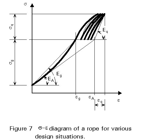
From this Figure three values of the modulus of elasticity can be observed:
For the first loading Eg = sg / eg
For the traffic loading Eq = sq / eq
For the total behaviour EA = sg / eA
It is clear that while the value of Eq remains almost constant, the value of Eg decreases as sg increases towards the overall stress sg + sq, while the opposite happens for EA.
Coupling, saddling and anchorage of cables are the three most important types of connections that occur in these structures (Figure 8); the requirements for these are as follows:
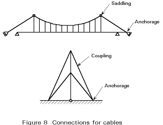
Examples of connections are given in Figure 9.
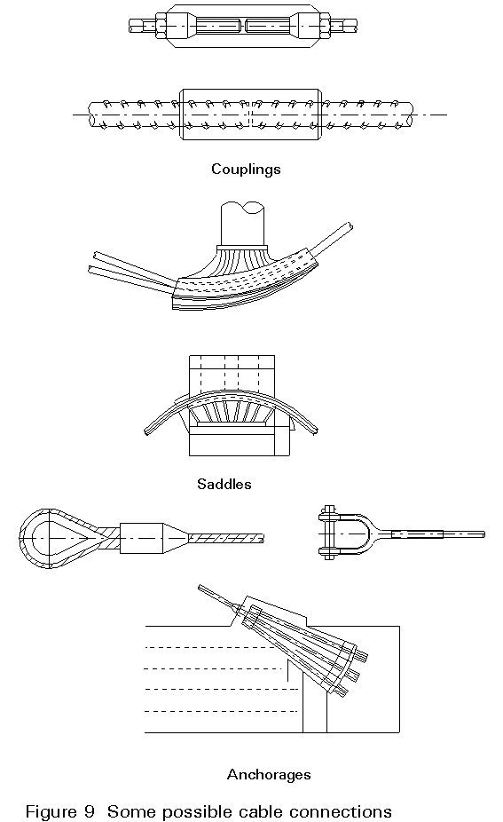
Figure 10 shows a cable which is suspended over two points, A and B, at different heights.
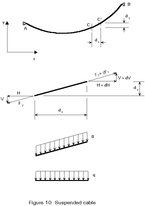
In order to derive the equations for this cable a small element CC¢ is cut off, and the forces at its ends together with the load acting on it are substituted in order to restore equilibrium; the two loading conditions considered here are:
g = a uniform load related to the inclined length.
q = a uniform load related to the horizontal projection.
It is further supposed that the cable has no bending stiffness, and can therefore only transmit axial loads.
The equilibria for the two loading cases are as follows:
Condition |
g |
q |
|
S H = 0 |
H - (H + dH) = 0 ® |
H = const |
(5) |
S M = 0 |
Vdx - Hdy = 0 ® |
V = Hy¢ ® V¢ = Hy² |
(6) |
S V = 0 |
V - (V + dV) + g ds = 0 |
V - (V + dV) + q dx = 0 |
|
® V¢ = g.ds / dx |
V¢ = q |
(7) |
(5), (6), (7) ® Hy² = g![]() (8a)
Hy² = q
(8b)
(8a)
Hy² = q
(8b)
Solution:
y = |
y = |
(9) |
Catenary |
Parabola |
|
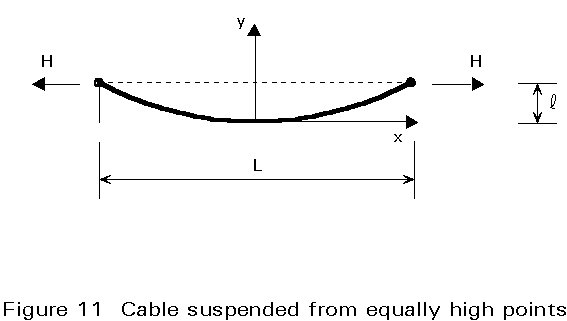
The coefficients C1 and C2 may be determined from the boundary conditions. For the special case of a cable suspended from two equally high points (Figure 11) the following expressions may be obtained:
|
g |
q |
|
|
|
|
(10) |
|
Tensile force Ft = H cosh |
|
(11) |
|
Cable length |
|
|
|
= |
= L + L |
(12) |
|
Sag |
|
(13) |
|
|
|
|
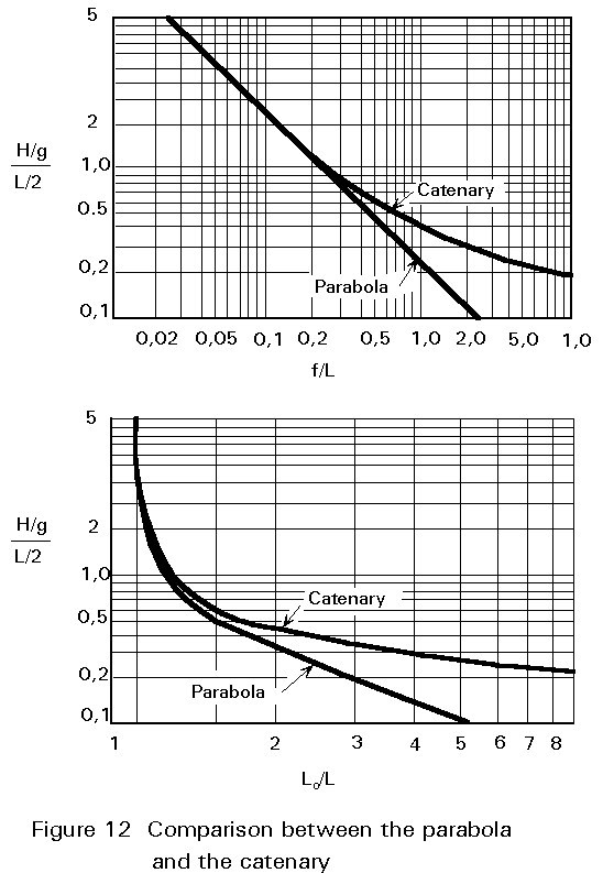
A comparison of the values given for sag and cable length by the two approaches is given in Figure 12; it can be seen that the catenary can be reasonably substituted by a parabola when the sag is small relative to the span; this is normally the case in guyed masts, cable stayed bridges, cranes etc. For other cases (e.g. transmission towers) the catenary should be used. Figure 12 shows that the approximation for the cable length is not as good as for sag.
For transmission towers two design situations (Figure 13) should normally be verified:
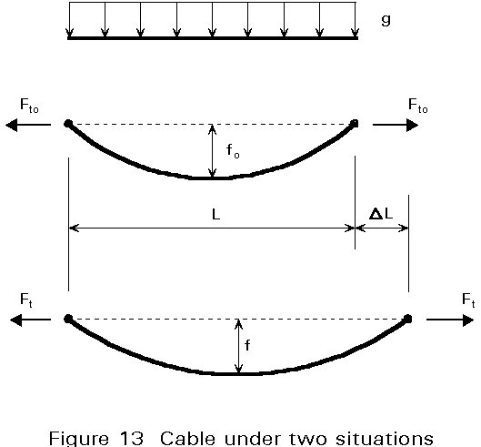
Winter situation: The cable is loaded by its self weight and the weight of the surrounding ice and the temperature is low, (t=-5° C)
Summer situation: The cable is loaded by its self weight and the temperature is high (t = 40° C).
The first situation yields the highest stress in the cable, whereas the second may be decisive for sag control. The governing equation for the verification is:
(s / E a) + t + (L2 g2 / 24s2) = const (14)
where:
s
is the stress in the cable.L is the span.
g
is the specific weight of the cable possibly including ice.t is the temperature.
E and a are the modulus of elasticity and the coefficient of thermal expansion of the cable.
The first term of Equation (14) expresses the strain of the cable due to the tensile force, the second the strain due to temperature and the third the strain due to sag.
When considering a cable whose end B moves from an initial position B to B¢ the following expressions are valid:
![]() (15)
(15)
The cable length, according to Equation (12), is equal to:
 (16)
(16)
which gives the displacement of point B as equal to:
![]() (17)
(17)
The longitudinal modulus of elasticity, due to sagging, is then equal to (Figure 14):
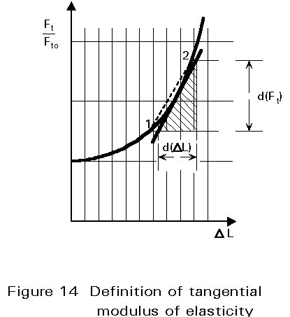
![]() (18)
(18)
The equivalent modulus of elasticity is then derived regarding both the elastic and the sagging deformations:
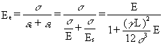 (19)
(19)
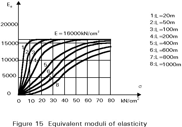
The value of Ee is dependent on the stress levels presented in Figure 15. The figure shows that short cables, subjected to high stresses, behave like the steel parent material, whereas long cables, subjected to small stresses, are much less stiff; this is one of the reasons why cable structures must be prestressed as otherwise they would be subjected to very large deformations.