ESDEP WG 12
FATIGUE
This lecture contains the background information of the basis of the Eurocode 3 rules concerning the fatigue design of structural elements.
None.
Lecture 12.1: Basic Introduction to Fatigue
Lecture 12.2: Advanced Introduction to Fatigue
The lecture discusses the main fatigue design rules contained in Eurocode 3 [1]. These fatigue design rules are based on fatigue test results obtained mainly under constant amplitude loading. The classification of a given detail, either welded or bolted, results from a statistical evaluation of the fatigue test data with a 95% probability of survival for a 75% confidence interval. The evaluation is compared with a set of equally spaced S-N curves with a slope constant of m = 3.
Explanation is given on the choice of a normalised double-slopes S-N curve. Then several factors, introduced in Eurocode 3 [1], affecting the fatigue strength are also discussed.
The principal objective of this lecture is to review the main rules which are the basis for Chapter 9 of Eurocode 3 [1] concerning the fatigue strength assessment of steel structural details.
The main provisions of Eurocode 3 [1] rely upon a set of fatigue resistance curves, equally spaced, upon which are classified a set of constructional details. The concept for fatigue strength design follows the Recommendations of the European Convention for Constructional Steelwork (ECCS). The Recommendations [2] define a set of equally spaced fatigue strength curves with a constant slope of m = 3 (for normal stress), or m = 5 (for shear stress, hollow section joints, and some particular details).
In addition to this approach another concept supported mainly by recent developments and research in the field of fatigue for "offshore" structures is referred to in Eurocode 3 as the geometrical stress concentration concept (also called the "hot spot stress" method).
To determine the fatigue strength provisions given in Eurocode 3, a compilation of fatigue data of various sources was carried out. This work has provided an opportunity to re-evaluate existing fatigue test data and allowed for a more consistent approach to the classification of detail categories.
Fatigue of steel structural components, especially welded steel details, is a particularly complex problem, and many factors may exert an influence on the fatigue life. Table 1 lists a non-exhaustive inventory of these various factors and those which are taken into account either explicitly or implicitly in Chapter 9 of Eurocode 3 are indicated.
Whilst some factors are dealt with in Chapter 9 of Eurocode 3, other factors, particularly those related to fabrication are considered in an implicit manner through defined discontinuities or weld defects acceptance criteria and quality control requirements. These general requirements will be defined in a standard concerning the "Execution of steel structures".
Table 1 The main factors affecting fatigue strength
|
Designation of the factors affecting the fatigue strength |
Taken into account in Eurocode 3 |
|
Stress × Stress or strain range × Stress sequence × Frequency (no significant effect when < 40 Hz in a non corrosive environment) × Mean stress (no effect in heat affected zone due to residual stresses) × Residual stresses |
*
* * |
|
Geometry × Nominal or geometrical stress × Local stress concentration × Small discontinues - scratches - grinding marks - surface pittings - weld defects or misalignments × Size effect (or scale effect) |
* * *(implicit)
* |
|
Material Properties and Fabrication × Stress-strain behaviour of materials × Hardness × Chemical composition of steels × Metallurgical homogeneity × Electrical potential × Micro structural discontinuities (grain size, grain boundaries) × Welding process × Weld heat treatment × Weld surface treatment |
|
|
Environment × Corrosive atmosphere × Temperature × Humidity (hydrogen embrittlement) × Irradiation |
*(implicit) *(implicit) |
In the preparation of Eurocode 3, classification into detail categories was established from a statistical analysis of fatigue test data obtained from various laboratory sources. To obtain more homogeneous samples of the test results, particular attention was paid to failure criteria considered in these tests.
Several failure criteria may be adopted to characterize the experimental failure condition at the end of a fatigue test in the laboratory. Three criteria are generally considered:
Generally for small scale specimens, the difference between the fatigue life at complete fracture and at a more realistic tolerable fatigue crack size is negligible. However, in a large scale structural element tested in fatigue the difference may be highly significant.
In Eurocode 3, the fatigue strength refers to the complete failure of the structural element. This condition corresponds, usually, to the criterion generally adopted by structural laboratories or reported in literature.
Different stresses may affect the fatigue strength classification of a structural detail. For a particular detail, the various origins of stresses have to be identified in order to define more precisely the design stresses for the fatigue assessment concepts involved in Chapter 9 of Eurocode 3.
a. Nominal Stress
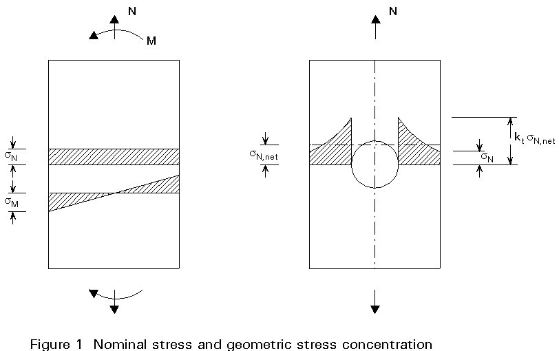
Consider a uniform structural member subjected to a simple axial force or to a bending moment. The nominal stress is the stress resultant calculated according to the basic strength of material (Figure 1).
The nominal stress of a member under uni-axial stress is:
sN = ![]() (2.1)
(2.1)
where N is the normal force and A the gross section area.
For a prismatic member section under a bending moment, the stress resultant is:
sM = ![]() (2.2)
(2.2)
where:
M is the applied bending moment
I is the moment of inertia of the section
v is the distance from the neutral axis to the outmost fibre.
b. Stress concentration effect due to geometrical discontinuities
There are three main sources which can create a state of stress concentration in a structural detail:
× The global geometry of the structural element which contains the structural detail, e.g. attachments on a beam web or gusset plates on a beam flange.
× The local stress concentration due to local disturbance of the weld geometry, bolt holes, local variation in stiffness, etc... For example, if a hole is drilled in a plate, the stress distribution across the section containing the hole will be different from the nominal stress distribution existing in the plain plate cross-section. An important stress gradient will occur in the vicinity of the hole. This geometrical stress concentration is due to both the decrease from the gross section to the net section and to the stress "raiser" (concentrator) caused by the presence of the hole (Figure 1).
× The local stress concentration due to local discontinuities occurring during fabrication (misalignment, surface scratch, pitting, weld defect, etc).
In many cases, and by simplification, the geometric stress concentration is usually calculated on the basis of the nominal stress applied to the gross section area and the stress concentration factor kG, as:
sG = kG . snom (2.3)
This structural geometrical stress concentration, which is defined as the maximum principal stress existing in the vicinity of the detail, may be evaluated from experimental tests or from finite element methods.
The local stress concentration is present in addition to the structural geometric stress concentration and may be due to local disturbances of the local geometry of the detail such as:
× local cross-section change (geometry of welds for example).
× local geometrical imperfections such as misalignment.
× small local discontinuities inherent to the action of the environment or of the fabrication process such corrosion pits, surface scratches, drag lines due to flame cutting, grinding marks, welding process defects such as undercut, lack of penetration, lack of fusion, slag inclusions, porosities, hydrogen-induced cracking, etc. These very small discontinuities are present in every element of engineering structures. Their presence determines a potential location for initiation of a fatigue crack.
Local stress concentrations are taken into account in an implicit manner in the derivation of the S-N curve from fatigue test results. Great care must be taken when assessing fatigue strength from tests on small scale specimens instead of large scale specimens. The scale effect due to weld geometry may have a greater influence on the fatigue strength in small test specimens than in large test specimens.
Usually, fatigue specimens have been tested with inherent discontinuities, and fatigue strength curves, so derived, make allowance for tolerable defects. The acceptance criteria for weld discontinuities which will be proposed in the "Execution of steel structures" standard would guarantee the fitness for purpose of the fatigue strength design rules of Eurocode 3. In other words, the quality assurance system which covers the fabrication process should ensure that the fabricated constructional detail complies with the relevant quality requirement specified in the standard for the "Execution of steel structures".
When assessing the fatigue strength by the so-called geometric stress range method, according to Clause 9.5.3 of Eurocode 3, the geometric stress concentration as defined by Equation (2.3) must be properly evaluated. The local geometry of the weld must not be taken into account in the calculation procedure of the design stress range, since the local discontinuity effect is already introduced in the derivation of the S-N curves. However, when determining the design stress, secondary stresses arising from joint eccentricity or due to joint stiffness, stress redistribution due to buckling or shear lag, and effects such as prying action, should be taken into account.
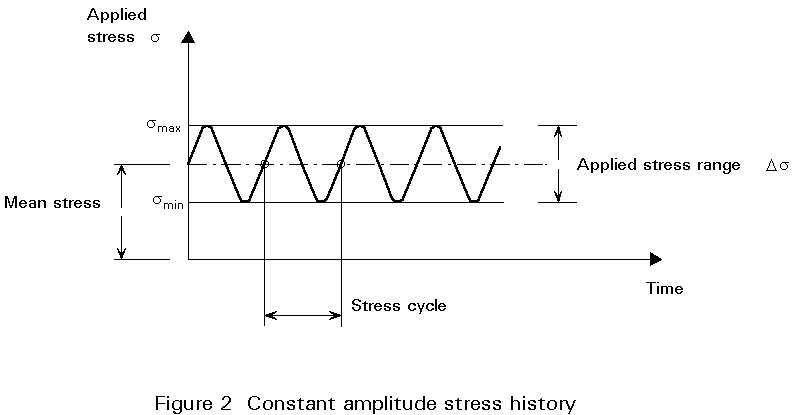
A fluctuating stress to which a structural detail is subjected may have a stress history of constant amplitude or of variable amplitude (Figures 2 and 3).
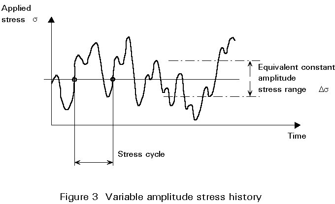
For cumulative damage analysis, the stress history is split up into individual cycles and related stress ranges which are summed up to a distribution of stress ranges. This distribution of stress ranges is called a stress spectrum, see Lecture 12.2.
For a variable amplitude stress history, there is a need to define such a stress cycle associated with a particular stress range. There are several procedures for cycle counting methods. Eurocode 3 refers to the "reservoir method" which gives a sound representation of the stress variation characteristic by allowing a proper contribution of each stress range to the fatigue damage process. This stress range counting method is the most commonly accepted. This counting method is somewhat similar to the well known "rainflow counting method". The "rainflow" and the "reservoir" counting methods do not lead to exactly the same result. However, in terms of fatigue damage both counting procedures give very close results, and for "long" stress histories they give nearly the same result.
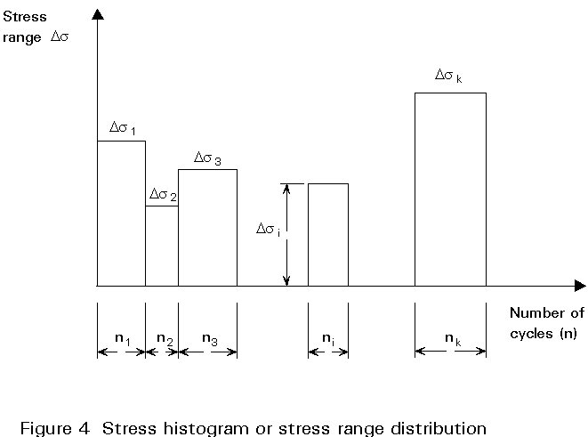
The most common way of representing irregular stress histories for fatigue analysis is to sum up the stress ranges of equal amplitude, and to obtain a distribution of stress range blocks which is called a stress histogram (or a stress spectrum) consisting of a number of constant stress range blocks. Each block is characterized by its number of cycles ni and stress range Dsi (Figure 4). The ordering of the different blocks does not make any difference since the damage calculation rules specified in Eurocode 3 refers to the linear cumulative damage rule of Palmgren-Miner. However for convenience the stress histogram is commonly presented with stress blocks ranked in decreasing order (Figure 5) which often can be approximated by a two-parameters Weibull distribution such as:
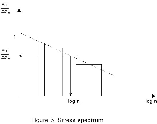
Ds
= Ds0 (2.4)
(2.4)
The classified fatigue design curves adopted in Eurocode 3, are the same as proposed in the "European Convention for Construction Steelwork Fatigue Recommendations" [2]. The ECCS Fatigue Recommendations were one of the first attempts to provide uniformity to the determination of the fatigue strength design curves.
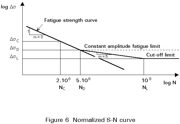
The ECCS Recommendations define a set of equally spaced S-N curves plotted on a log-log scale. Reference to these curves allows a detail category to be classified (representative) of a particular structural detail which corresponds to a notch effect or a characteristic geometrical discontinuity). This classification has been determined by a series of fatigue test results, from which a statistical and a probabilistic evaluation is performed, see Lecture 12.7.
Each individual fatigue strength curve is defined in a conventional way (Figure 6) by a slope constant of m = 3 (slope = -1/3). The constant amplitude limit is set at 5 million cycles. The slope constant m = 3 was a best fit for a large number of different structural details tested in fatigue. The figure of 5 million cycles for the constant amplitude fatigue limit is a compromise between 2 million cycles for "good" details and 10 million cycles for details which create a severe notch effect. For any stress range of constant amplitude below this limit, no fatigue damage is expected to occur.
When a detail is subjected to variable stress ranges, which is generally the case in reality, several options may occur:
In this last option, two cases have to be considered for the cumulative damage calculation when some stress ranges are below the constant amplitude fatigue limit:
In both cases, all cycles below cut-off limit can be ignored when evaluating the fatigue damage. It should be noted that Eurocode 3 leaves the design engineer free to use either the single-slope S-N curve or the double-slope S-N curve.
Experimental results have indicated that within the range of high numbers of cycles, a change in the slope of the fatigue strength occur due to a decrease of the crack growth rate. The introduction of a double-slope concept and a constant amplitude fatigue limit at 5 million cycles is still a matter of controversy. Despite a number of criticisms, particularly concerning the increase in complexity of the analysis, Eurocode 3 has kept the double-slope curve because this rule may, for some detail categories, improve the accuracy of the fatigue check. However, this improvement can not expected for all types of structural detail, and all stress spectra. In some cases, especially for those details with a very severe notch effect, the double-slope curve may not lead to a conservative result.
Some details, for example, cover-plated beams, have shown a constant amplitude fatigue limit of almost 10 million cycles. To avoid non-conservative conditions, some details (which generally have severe notch effect) have been classified in categories slightly lower than their fatigue strength at 2 million cycles would have required. The concept of the specified ECCS fatigue design curves, which consists of 14 equally spaced curves, a new design fatigue strength curve is not required for each new structural detail.
The "grid system" of S-N curves has been established as follows. The vertical distance of the ordinate log-scale between each fatigue strength curves has been obtained by dividing the difference between one order of magnitude into 20 equal spaces (Figure 7). For example, taking two reference values as Dsc=100MPa and Dsc = 1000 MPa at 2 million cycles, the calculation of the spacing is determined from the following:
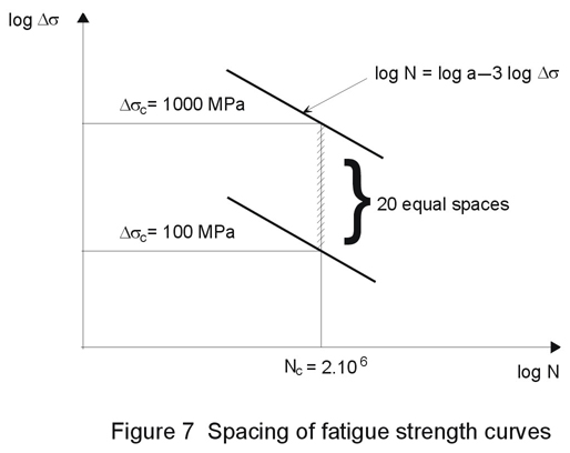
The general S-N curve equation may be written as:
log N = log a - 3 log Ds (4.1)
so with Dsc = 100 MPa (log 2 000 000 = 6,30103)
log a = 6,30103 + 3 log 100 = 12,301 (4.2)
and for Dsc = 1000 MPa
log a = 6,30103 + 3 log 1000 = 15,301 (4.3)
The spacing between two contiguous curves represents
D
log a = (15,301 - 12,301)/20 = 0,15 (4.4)So starting from the reference values of Dsc = 100 MPa, with log a = 12,301, the subsequent values of Dsc may be obtained from Equation (4.1) as given in Table 2.
Table 2 Characteristic fatigue strength at 2 million cycles
|
log a |
Ds c (rounded value) |
|
... 12,601 12,451 12,301 12,151 12,001 ... |
... 125 112 100 90 80 ... |
Table 2 shows that the number defining the characteristic fatigue strength at 2 million cycles, used as a detail category identification, is a rounded value.
Generally fatigue strength curves are evaluated from series of fatigue tests performed on specimens which typically reproduce the detail to be studied. The fatigue strength curves (S-N curves) can be most accurately determined when a group of fatigue specimens are tested at different stress range levels. However, there is no recognized standard method for fatigue testing and design experiments. As a result, the fatigue test data found in the literature are somewhat non-homogeneous.
It is clear that, under such circumstances, a review of existing fatigue data and their statistical evaluation, even when limited to the same detail category, may lead to large discrepancies in the results. Such differences may be attributed, not only to the fatigue testing practice in each laboratory, but also to the detailed fabrication procedure and quality achieved in the preparation of the specimens. Discontinuities play a major role in fatigue strength, particularly for welded details and careful consideration must be given to the weld quality which may considerably affect the variation in fatigue strength.
Fatigue specimens are fabricated with certain inherent discontinuities which are not fully known or may not be properly evaluated in laboratory reports. In such cases, it is generally rather difficult to appreciate if the fabrication quality of specimens is representative of current workshop practice. Moreover, when performing a statistical analysis on fatigue test data from different origins, a rather large variation of fatigue strength may result. Careful attention must be paid to the homogeneity of the fatigue resistance.
These considerations were borne in mind during the preparation of Eurocode 3. The fatigue test results which were statistically analyzed and then classified according to the procedure described fulfil certain requirements:
In real life, structural elements are subjected to varying fatigue loads, and not to constant amplitude fatigue loadings. Eurocode 3 refers to the Palmgren-Miner summation to evaluate the cumulative damage (Figure 8). This rule is based on the assumption that the total damage accumulated by a structural element under varying stress ranges, is obtained by the linear summation of the damage of each individual stress range, i.e:
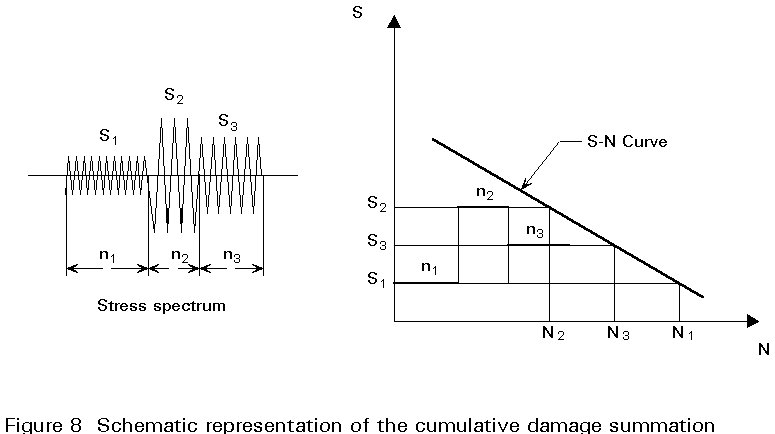
D = ![]() (6.1)
(6.1)
where:
ni is the number of cycles of constant amplitude stress ranges Dsi
Ni is the total number of cycles to failure under constant amplitude stress range Dsi.
The structural element is designed safely against fatigue if:
D £ 1 (6.2)
No account of the damage is taken for any varying stress ranges falling below the cut-off limit.
The concept of equivalent stress range has been introduced in the ECCS Recommendations [2] and is also referred to in Eurocode 3. The definition of the equivalent stress range is conventional. It can be said that the equivalent stress range concept is simpler than a direct Palmgren-Miner summation when the S-N curve is of unique slope (-1/m). The expression is, in this case, quite simple and the recalculation of the damage for each S-N curve is therefore avoided:
Ds
equ = (6.3)
(6.3)
with m = 3 or m = 5 as appropriate.
The equivalent stress range Dsequ depends only on the fatigue load spectrum and the slope constant m. In such a case, knowing Dsequ evaluated according to Equation (6.3), it is easy to choose directly a detail category which will have an adequate fatigue resistance.
When the basic S-N curve is of double slope, the expression of the equivalent stress range becomes more unwieldy. The practicability of its application is questionable, except if using the limit state function as defined by the following equation:
g
f . Dsequ £ DsRd / gf (6.3)The derivation of Dsequ when the S-N curve has a double slope is given below:
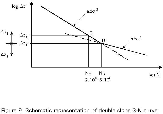
a. Damage calculation for a double slope S-N curve when the stress range is below and above DsD
Suppose there are some stress range blocks where the range is below the value of DsD and some above DsD (Figure 9); it is assumed that the proper partial safety coefficients have introduced in Dsi and Dsj.
× block i when Dsi > DsD
× block j when Dsj > DsD
From the definition the damage is given by:
D = ![]() (6.5)
(6.5)
taking into account the S-N curve slope for each set of stress range blocks:
D = ![]() (6.6)
(6.6)
Equation (6.6) may be written as:
D = ![]() (6.7)
(6.7)
From Figure 9:
ND = a DsD-3 = b DsD-5
ND corresponds to the fatigue limit of the S-N curve at 5 million cycles.
a/b = 1/DsD2 (6.8)
Hence:
D = ![]() (6.9)
(6.9)
where:
Q = S ni Dsi3 + S nj Dsj3 (Dsj /DsD)2
The damage may be calculated using either Equation (6.5) or Equation (6.9) directly.
b. Calculation of the equivalent stress range Dsequ for a double slope S-N curve
In this particular case, a decision must be made as to which slope the definition of Dsequ refers. The choice of a slope constant of 3 or 5 makes absolutely no difference to the final result of the calculation of Dsequ when the load spectrum straddles both parts of the double slope S-N curve. The calculation of the equivalent stress range Dsequ is derived below from a slope constant of m = 3 of the double slope S-N curve (noted as Dsequ.3). The same demonstration holds for a slope constant of m = 5. By definition:
D = ![]() (6.10)
(6.10)
where:
Nequ is the equivalent number of cycles at failure under the equivalent stress range Dsequ
N is equal to S ni + S nj
Evaluating Nequ on the basis of the S-N curve of slope constant m=3:
D = ![]() (6.11)
(6.11)
by equating Equations (6.6) and (6.11), the damage is:
D = ![]() (6.12)
(6.12)
then Equations (6.11) and (6.12) give:
Dsequ3 =  (6.13)
therefore:
Dsequ.3 =  (6.14)
DsRd.3 is defined as the fatigue resistance corresponding to Dsequ.3 on the S-N curve of constant slope m = 3.
DsRd.3 = DsD (ND / N)1/3 (6.15)
From Equations (6.14) and (6.15):
 =
= ![]() =
= ![]() (6.16)
(6.16)
This expression is equal to the damage as given by Equation (6.9):
= ![]() (6.17)
(6.17)
Remarks:
N (DsRd)m = a = constant
another reference value may be taken, for example:
DsD3 ND = DsC3 NC = constant
DsC, being the stress range at NC = 2 million cycles.
Welded joints in structural details contain tensile residual stresses in the vicinity of the weld bead. Figure 10 shows that their magnitude may be as high as the yield stress of the weldment metal. Figure 10 also shows high tensile residual stresses near the edges which were flame-cut.

It is well established that the presence of residual stresses of such magnitude makes the fatigue strength of a welded joint independent of the applied load ratio, and dependent only on the applied stress range. The full significance of the tensile residual stresses due to welding was not appreciated originally, since many fatigue test results were obtained from welded specimens which were too small to retain the major part of the welding residual stresses such as would occur in large structural components.
It is evident that tensile stresses play a significant role in the propagation of a crack, since they tend to act as a opening mode due to tensile stresses applied at the crack lips. The crack propagation rate is likely to be reduced, when the crack grows into a zone of compression residual stress.
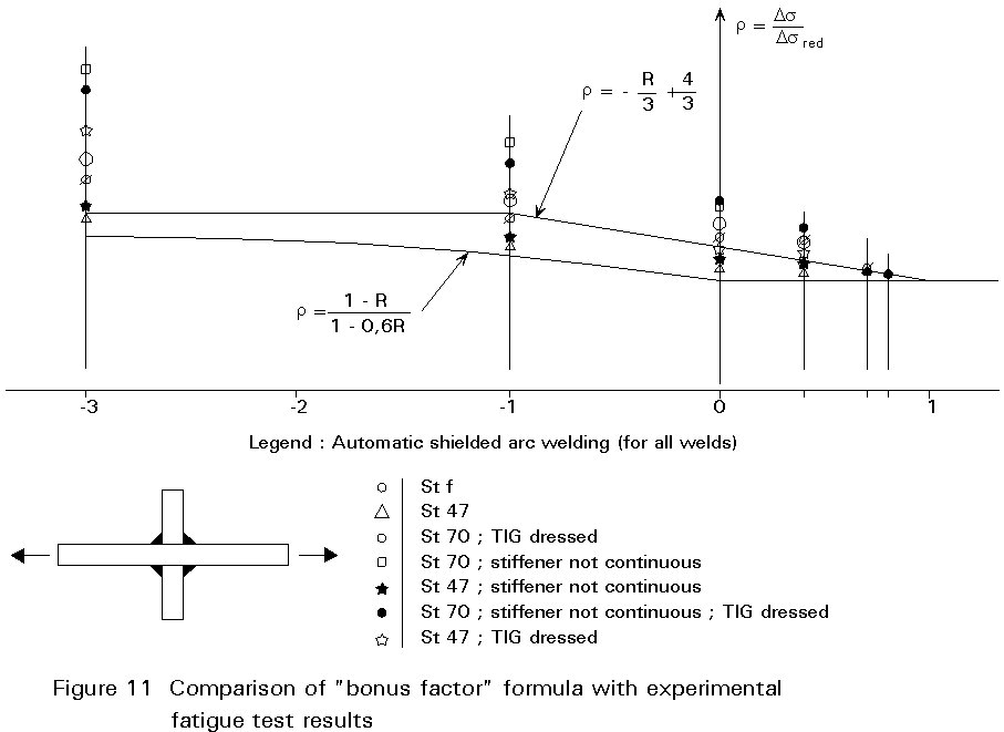
It is in recognition of this physical crack propagation behaviour that the R ratio (R = smin/smax) has been considered in Eurocode 3 Chapter 9 for non-welded or stress relieved details. Figure 11 shows the comparison between fatigue test results and two "bonus factor" rules which were studied when drafting Chapter 9. The rule which was finally selected takes into account of the effect of compressive stress ranges by multiplying the part of the stress range in compression by a factor of 0,6. The validity of this rule has been compared with fatigue test results performed on non-load carrying weld cruciform joints for various R ratios ranging from -3,0 to 0,8. These fatigue tests were carried out on small specimens.
[1] Eurocode 3: "Design of Steel Structures": ENV1993-1-1: Part 1.1, General rules and rules for buildings, CEN, 1993.
[2] European Convention for Constructional Steelwork: Recommendations for the Fatigue Design of Steel Structures. ECCS Publication 43, 1985.
[3] Eurocode 1: "Basis of Design and Actions on Structures", CEN (in preparation).