ESDEP WG 12
FATIGUE
To introduce the main concepts and definitions regarding the fatigue process and to identify the main factors that influence the fatigue performance of materials, components and structures.
Lecture 12.1: Basic Introduction to Fatigue
The physical process of the initiation of fatigue cracks in smooth and notched test specimens under the influence of repeated loads is described and the relevance of this process for the fatigue of real structures is discussed.
The basis of different stress cycle counting procedures is explained for variable amplitude loading. Exceedance diagram and frequency spectrum effects are described.
Fatigue is commonly referred to as a process in which damage is accumulated in a material undergoing fluctuating loading, eventually resulting in failure even if the maximum load is well below the elastic limit of the material. Fatigue is a process of local strength reduction that occurs in engineering materials such as metallic alloys, polymers and composites, eg. concrete and fibre reinforced plastics. Although the phenomenological details of the process may differ from one material to another the following definition given by ASTM [1] encompasses fatigue failures in all materials:
Fatigue - the process of progressive localised permanent structural change occurring in a material subjected to conditions that produce fluctuating stresses and strains at some point or points and that may culminate in cracks or complete fracture after a sufficient number of fluctuations.
The important features of the process relevant to fatigue in metallic materials are indicated by the underlined words in the definition above. Fatigue is a progressive process in which the damage develops slowly in the early stages and accelerates very quickly towards the end. Thus the first stage consists of a crack initiation phase, which for smooth and mildly notched parts that are subjected to small loads cycles may occupy more than 90 percent of the life. In most case cases the initiation process is confined to a small area, usually of high local stress, where the damage accumulates during stressing. In adjacent parts of the components, with only slightly lower stresses, no fatigue damage may occur and these parts thus have an infinite fatigue life. The initiation process usually results in a number of micro-cracks that may grow more or less independently until one crack becomes dominant through a coalescence process at the microcracks start to interact. Under steady fatigue loading this crack grows slowly, but starts to accelerate when the reduction of the cross-section increases the local stress field near the crack front. Final failure occur as an unstable fracture when the remaining area is too small to support the load. These stages in the fatigue process can in many cases be related to distinctive features of the fracture surface of components that have failed under fluctuating loads, the presence of these features can therefore be used to identify fatigue as the probable cause of failure.
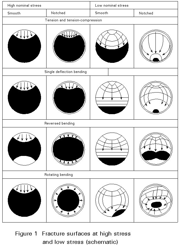
Typical fracture surfaces in mechanical components that were subjected to fatigue loads are shown in Slide 1. One characteristic feature of the surface morphology which is evident in both macrographs is the flat, smooth region of the surface exhibiting beach marks (also called clamshell marks). This part represents the portion of the fracture surface over which the crack grew in a stable, slow mode. The rougher regions, showing evidence of large plastic deformation, is the final fracture area through which the crack progressed in an unstable mode. The beach marks may form concentric rings that point toward the areas of initiation. The origin of the fatigue crack may be more or less distinct. In some cases a defect may be identified as the origin of the crack, in other cases there is no apparent reason why the crack should start at a particular point in a fracture surface. If the critical section is at a high stress concentration fatigue initiation may occur at many points, in contrast to the case of unnotched parts where the crack usually grows from one point only see Figure 1. While the presence of any defects at the origin may indicate the cause of the fatigue failure, the crack propagation area may yield some information regarding the magnitude of the fatigue loads and also about the variation in the loading pattern. Firstly, the relative magnitude of the areas of slow-growth and final fracture regions give an indication of the maximum stresses and the fracture toughness of the material. Thus, a large final fracture area for a given material indicates a high maximum load, whereas a small area indicates that the load was lower at fracture. Similarly, for a fixed maximum stress, the relative area corresponding to slow crack growth increases with the fracture toughness of the material (or with the tensile strength if the final fracture is a fully ductile overload fracture).
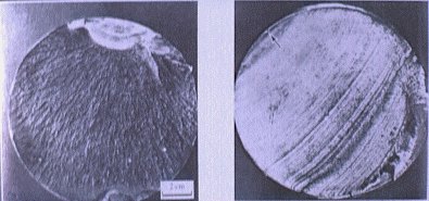
Slide 1 : Typical fatigue failures in steel components.
Beach marks are formed when the crack grows intermittently and at different rates during random variations in the loading pattern under the influence of a changing corrosive environment. Beach marks are therefore not observed in the surfaces of fatigue specimens tested under constant amplitude loading conditions without any start-stop periods. The average crack growth is of the order of a few millimetres per million cycles in high cycle fatigue, and it is clear that the distance between bands in the beach marks are not a measure of the rate of crack advance per load cycle. However, examination by electron microscope at magnifications between 1,000x and 30,000x may reveal characteristic surface ripples called fatigue striations, see Slide 2. Although somewhat similar in appearance, these lines are not the beach marks described above as one beach mark may contain thousands of striations. During constant amplitude fatigue loading at relatively high growth rates in ductile material such as stainless steels and aluminium alloys the striation spacing represents the crack advancement per load cycle. However, in low stress, high cycle fatigue where the striation spacing is less than one atomic spacing (- 2.5 x 10⁻⁸m) per cycle. Under these conditions the crack does not advance simultaneously along the crack front, growth occurring instead only along some portions during a few cycles, then arrests while growth occurs along other segments. Striations as shown in Figure 3 are not seen if the crack grows by other mechanisms such as microvoid coalescence or, in brittle materials, microclevage. In structural steels the crack can propagate by all three mechanism, and striations may be difficult to observe. Slide 3 shows an example of beach marks and striations in the fracture originating at a large defect in a welded C-Mn steel with a yield strength of about 360Mpa.
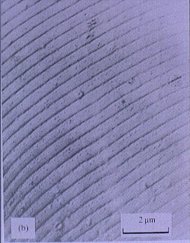
Slide 2 : Striations in an aluminium alloy.
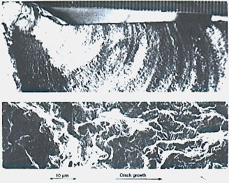
Slide 3 : Fatigue failures in the Alexander L Kielland platform.
From the description of the characteristics of fatigue fracture surfaces, three stages in the fatigue process may be identified:
Stage I: Crack initiation
Stage II: Propagation of one dominant crack
Stage III: Final fracture
Fatigue cracking in metals is always associated with the accumulation of irreversible plastic strain. The crack process which is discussed in the following applies to smooth specimens made of ductile materials.
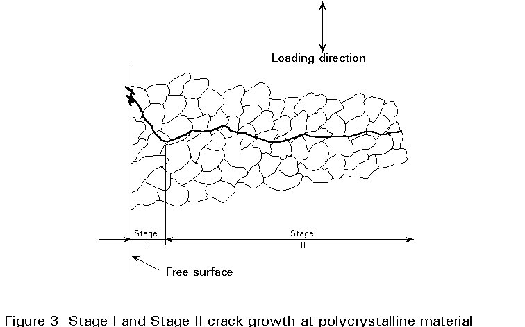
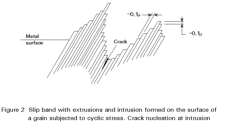
In high cycle fatigue the maximum stress in cyclic loads that eventually cause fatigue failure may be well below the elastic limit of the material, and large scale plastic deformation does not occur. However, at a free surface plastic strains may accumulate as a result of dislocation movements. Dislocations are line defects in the lattice structure which can move and multiply under the action of shear stresses, leaving a permanent deformation. Dislocation mobility and hence the amount of deformation (or slip) is greater at a free surface than in the interior of crystalline materials due to lack of constraint from grain boundaries. Grains in polycrystalline structural metals are individually oriented in a random manner. Each grain, however, has an ordered atomic structure giving rise to directional properties. Deformation for example, takes place on crystallographic planes of easy slip along which dislocations can move more easily than other planes. Since slip is controlled primarily by shear stress, slip deformation takes place along crystallographic planes that are orientated close to 45° to the tensile stress direction. The results of such deformation is atomic planes sliding relative to each other, resulting in a roughening of the surface in slip bands. During further cycling slip band deformation is intensified at the surface and extending into the interior of the grain, resulting in so-called persistent slip bands, (PSB's). The name originated from the observation in early studies of fatigue that slip band would reappear - "persist" - at the same location after a thin surface layer was removed by elastopolishing. The accumulation of local plastic flow result in surface ridges and troughs called extrusions and intrusions, respectively, Figure 2. The cohesion between the layers in slip band is weakened by oxidation of fresh surfaces and hardening of the strained material. At some point in this process small cracks develop in the intrusions. These microcracks grow along slip planes, ie. a shear stress driven process. Growth in the shear mode, called stage I crack growth extends over a few grains. During continued cycling the microcracks in different grains coalesce resulting in one or a few dominating cracks. The stress field associated with the dominating crack cause further growth under the primary action of maximum principal stress; this is called stage II growth. The crack path is now essentially perpendicular to the tensile stress axis. Crack advancement is, however, still influenced by the crystallographic orientation of the grains and the crack grows in a zigzag path along slip planes and cleavage planes from grain to grain, see Figure 3. Most fatigue cracks advance across grain boundaries as indicated in Figure 3, ie. in a transcrystalline mode. However, at high temperatures or in a corrosive environment, grain boundaries may become weaker than the grain matrix, resulting in intercrystalline crack growth. The fracture surface created by stage II crack growth are in ductile metals characterised by striations whose density and width can be related to the applied stress level.
Since crack nucleation is related to the magnitude of stress, any stress concentration in the form of external or internal surface flaws can marked reduce fatigue life, in particular when the initiation phase occupies a significant portion of the total life. Thus a part with a smooth, polished surface generally has a higher fatigue strength than one with a rough surface. Crack initiation can also be facilitated by inclusions, which act as internal stress raisers. In ductile materials slip band deformations at inclusions are higher than elsewhere and fatigue cracks may initiate here unless other stress raisers dominate.
In high strength materials, notably steels and aluminium alloys, a different initiation mechanism is often observed. In such materials, which are highly resistant to slip deformation, the interface between the matrix and inclusion may be relatively weak, and cracks will start here if decohesion occurs at the inclusion surface, aided by the increased stress/strain field around the inclusion. Slide 4 shows small fatigue cracks originating at inclusions in a high strength steel. Alternatively, a hard brittle inclusion may break and a fatigue crack may initiate at the edges of the cleavage fracture.
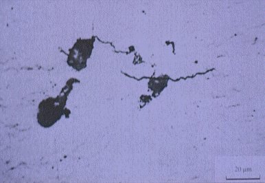
Slide 4 : Fatigue crack initiation at an inclusion in a high strength steel alloy.
From the discussion above it is evidently not possible to make a clear distinction between crack nucleation and stage I growth. "Crack initiation" is thus a rather imprecise term used to describe a series of events leading to stage II crack. Although the initiation stage includes some crack growth, the small scale of the crack compared with microstructural dimensions such as grain size invalidates a fracture mechanics based analysis of this growth phase. Instead, local stresses and strains are commonly related to material constants in prediction models used to estimate the length of stage I. The material constants are normally obtained from tests on smooth specimens subjected to stress or strain controlled cycling.
The simplest form of stress spectrum to which a structural element may be subjected is a sinusoidal or constant amplitude stress-time history with a constant mean load, as illustrated in Figure 4. Since this is a loading pattern which is easily defined and simple to reproduce in the laboratory it forms the basis for most fatigue tests. The following six parameters are used to define a constant amplitude stress cycle:
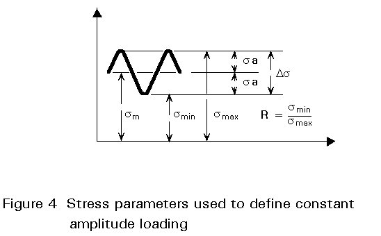
Smax = maximum stress in the cycle
Smin = minimum stress in the cycle
Sm = mean stress in the cycle = (Smax + Smin)/2
Sa = stress amplitude = (Smax Smin)/2
AS = stress range = Smax - Smin = 2Sa
R = stress ratio = Smin/Smax
The stress cycle is uniquely defined by any two of these quantities, except combinations of stress range and stress amplitude. Various stress patterns are shown in Figure 5, with definitions in accordance with ISO [2] terminology.
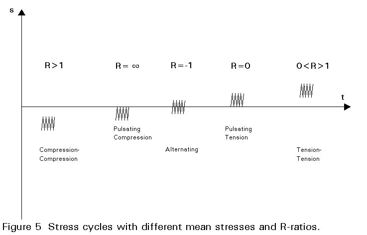
The stress range is the primary parameter influencing fatigue life, with mean stress as a secondary parameter. The stress ratio is often used as an indication of the influence of mean loads, but the effect of a constant mean load is not the same as for a constant mean stress. The difference between S-N curves with constant mean stress or constant R-ratio is discussed in the section on fatigue testing.
The test frequency is needed to define a stress history, but in the fatigue of metallic materials the frequency is not an important parameter, except at high temperatures when creep interacts with fatigue, or when corrosion influences fatigue life. In both cases a lower test frequency results in a shorter life.
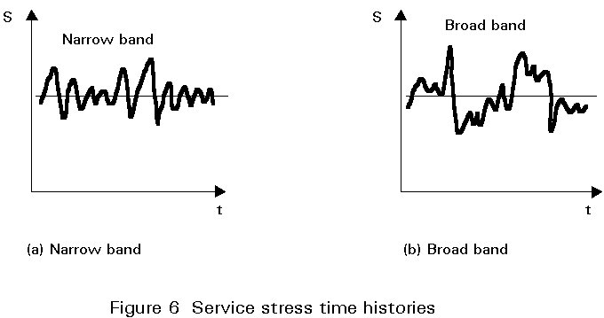
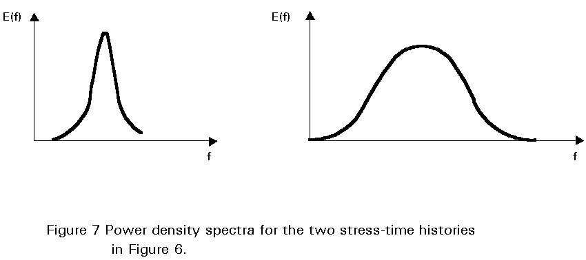
Typical stress-time histories obtained from real structures are one shown in Figure 6. The sequence in Figure 6a has a constant mean stress, individual stress cycles are easily identifiable, and it necessary to evaluate this stress history in terms of stress range only. The more "random" stress variations in Figure 10b is called a broad band process because the power density function (a plot of energy vs. frequency) spans a wide frequency range, in contrast to the one in Figure 6a which contains essentially one frequency. The difference is illustrated in Figure 7. The load history in Figure 6 can be interpreted as a variation of the main load with superimposed smaller excursions that could be caused by eg. second order vibrations or by electronic noise in the load acquisition system. In case of true mean load variations not only the range but also the mean of each cycle needs to be recorded in order to estimate the influence of mean load on the damage accumulation. In both cases it is necessary to eliminate the smaller cycles since they may be below the fatigue limit and therefore cause no fatigue damage, or because they do not represent real load cycles. Thus a more complicated evaluation procedure is required for identifying and counting individual major stress cycles and their associated mean stresses. Counting methods such as the range pair, rainflow and the reservoir methods are designed to achieve this. These procedures are described in paragraph 7.
The total fatigue life in terms of cycles to failure can be expressed as:
Nt = Ni + Np (1)
where Ni and Np are number of cycles spent in the initiation and propagation stages, respectively. As noted, the two stages are distinctly different in nature and different material parameters control their length. The life of unnotched components, for example, is dominated by crack initiation. In sharply notched parts, however, or in parts containing crack-life defects, eg. welded joints, the crack growth stage dominates and crack propagation data may be used in an assessment of fatigue life using fracture mechanics analysis. Therefore different test methods are necessary to assess the fatigue properties of these types of components.
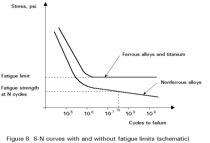
Fatigue data for components whose lives consist of an initiation phase followed by crack propagation are usually presented in the form of S-N curves, where applied stress S is plotted against total cycles to failure, N (= Nt). As the stress decreases, the life in cycles to failure increases, as illustrated in Figure 8. The S-N curves for ferrous and titanium alloys exhibit a limiting stress below which failure does not occur; this is called the fatigue or the endurance limit. The branch point or "knee" of the curve lies normally in the 105 to 107 cycle range. In aluminium and other nonferrous alloys there is no stress asymptote and a finite fatigue life exists at any stress level. All materials, however, exhibit a relatively flat curve in the high-cycle region, ie. at lives longer than about 105 cycles.
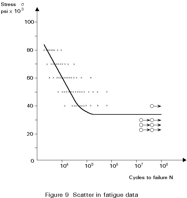
A characteristic feature of fatigue tests is the large scatter in fatigue strength data, this is particularly evident when a number of specimens are tested at the same stress level, as illustrated in Figure 9. Plotting the data for a given stress level along a logarithmic endurance axis gives a distribution which can be approximated by the Gaussian (or normal) distribution, hence endurance data are said to have a log normal distribution. Alternatively the Weibull distribution may be used, but the choice is not important since about 200 specimens, tested at the same stress level, are required to make a statistically significant distinction between the two distributions. This number is about one order of magnitude larger than the quantity of specimens that typically are available for fatigue testing at one stress level.
Assuming the life distribution to be log normal, the associated mean life curve and the standard deviation can be used to define a design S-N curve for any desired probability of failure.
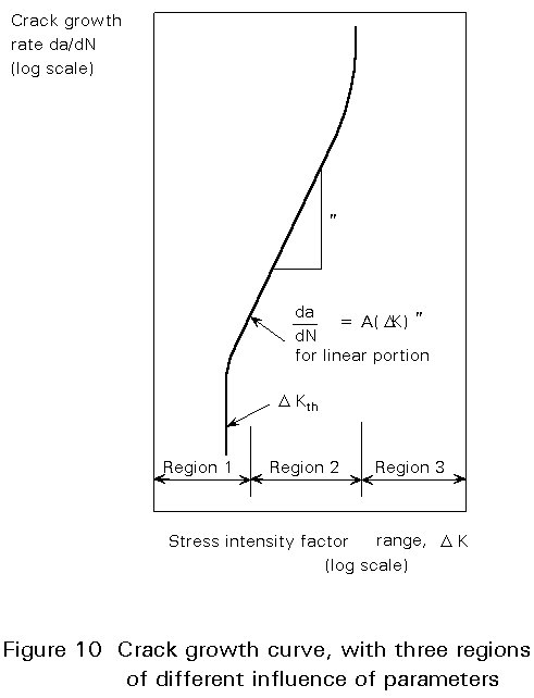
When the crack propagation stage dominates fatigue life, design data may be obtained from crack growth curves, an example of which is shown schematically in Figure 10. The stress intensity factor K uniquely describes the stress field near the crack tip, and is therefore used in the design against unstable fracture. Likewise, the range of the stress intensity factor, DK, may be expected to govern fatigue crack growth. The validity of this assumption was first proved by Paris [3], and later verified by many other researchers. The crack growth curve, which has a sigmoidal shape, spans three regions as indicated schematically in Figure 10. In Region I the crack growth rate drops off asymptotically as DK is reduced towards a limit or threshold, DKth, below which no crack growth takes place. Life fatigue endurance data, crack growth data show considerable scatter and test results must be evaluated by statistical methods in order to derive useful design data.
The basis for any design methodology aimed at preventing fatigue failures is data characterising the fatigue strength of components and structures. Fatigue testing is therefore essential for the fatigue design process. The ideal fatigue test may be defined as a test in which an actual structure is subjected to the service load spectrum of that structure. However, life estimates are required before the design is finalised or details of the loading history are known. Additionally, each structure will experience a particular load history that is unique for that structure, so many simplifications and assumptions need to be made regarding the test stress sequence which is going to represent the many types of service histories that can occur in practice.
Fatigue testing is therefore performed in several ways, depending on the stage the design or production of the structure has reached or the intended use of the data. The following four main types of tests can be identified:
The first three tests are idealised tests that produce information on the material response. The use of the results from these tests in life prediction of components and structures requires additional knowledge of influencing factors related to the geometry, size, surface condition and corrosive environment. S-N tests of components are also normally standardised tests that make life predictions more accurate compared with the three other tests because the uncertainties regarding the influence of notches and surface conditions are reduced. Service loading or variable amplitude testing normally requires a knowledge of the response of the actual structure to the loading environment, and is therefore normally used only for prototype or component testing at a late stage in the production process.
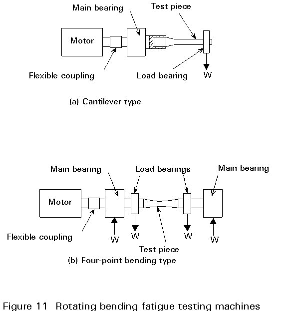
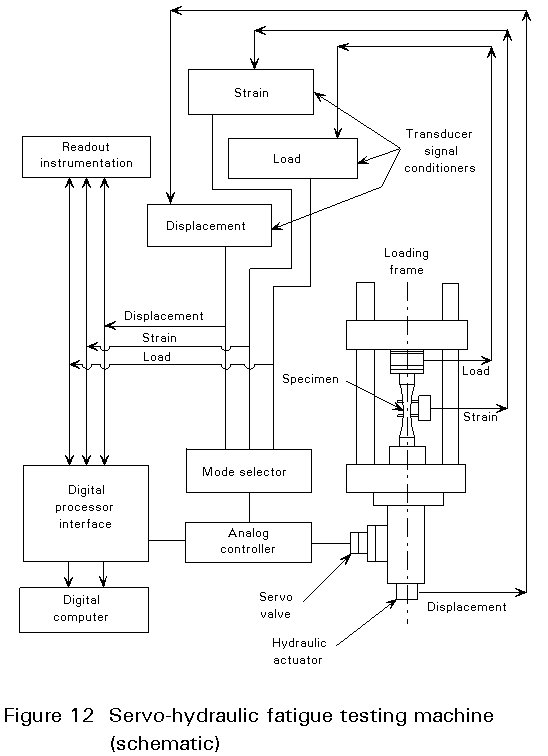
Rotating bending machines were used in the past to generate large amounts of test data in a relatively inexpensive way. Two types are shown schematically in Figure 11. The computer-controlled closed loop testing machines are widely used in all modern fatigue testing laboratories. Most are equipped with hydraulic grips that facilitate the insertion and removal of specimens. A schematic diagram of such a testing machine is shown in Figure 12. These machines are capable of a precise control of almost any type of stress-time, strain-time or load pattern and are therefore replacing other types of testing machines.
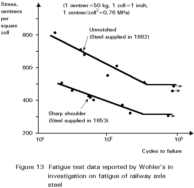
Among the first systematic fatigue investigations reported in the literature are those set up and conducted by the German railway engineer, August Wöhler, between 1852 and 1870. He performed tests on full scale railway axles and also small scale bending, axial and torsion tests on several types of materials. Typical examples of Wöhler's original data are shown in Figure 13. These data are presented in what is now well known as Wöhler or S-N diagrams. Such diagrams are still commonly used in the presentation of fatigue data, although the stress axis is often on a logarithmic scale in contrast to Wöhler's linear stress axis. Basquin's equation is often fitted to test data, it has the form:
Sa Nb = constant (2)
where Sa is the stress amplitude, and b is the slope. When both axes have logarithmic scales, Basquin's equation becomes a straight line.
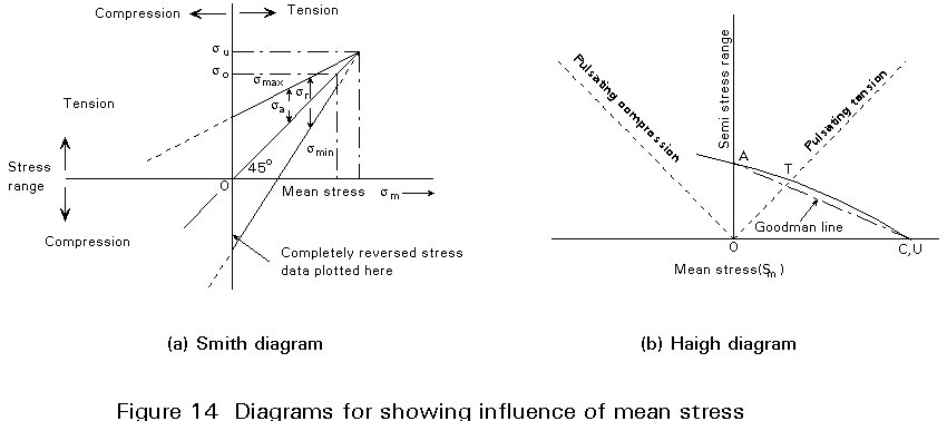
Other types of diagrams are used, for instance to demonstrate the influence of mean stress; examples are the Smith or Haigh diagrams which are shown in Figure 14. Low cycle fatigue data are almost universally plotted in strain vs. life diagrams since strain is a more meaningful and more easily measurable parameter than stress when the stress exceeds the elastic limit.
The difference in fatigue behaviour of full scale machine or structural components as compared with small laboratory specimens of the same material is sometimes striking. In the majority of cases the real life component exhibits a considerably poorer fatigue performance than the laboratory specimen although the computed stresses are the same. This difference in fatigue response can be examined in a systematic manner by evaluating the various factors that influence fatigue strength. Qualitative and quantitative assessments of these effects are presented in the following paragraphs.
Effect of static strength on basic S-N data
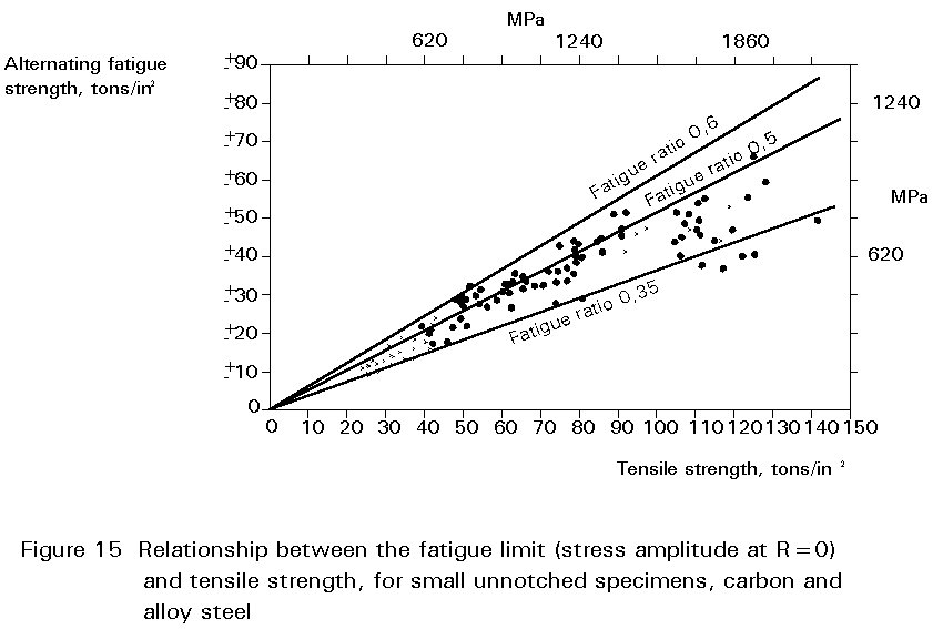
For small unnotched, polished specimens tested in rotating bending or fully reversed axial loading there is a strong correlation between the high-cycle fatigue strengths at 106 to 107 cycles (or fatigue limit) So, and the ultimate tensile strength Su. For many steel materials the fatigue limit (amplitude) is approximately 50% of the tensile strength, ie. So = 0.5 Su. The ratio of the alternating fatigue strength So to the ultimate tensile strength Su is called the fatigue ratio. The relationship between the fatigue limit and the ultimate tensile strength is shown in Figure 15 for carbon and alloy steels. The majority of data are grouped between the lines corresponding to fatigue ratios of 0.6 and 0.35. Another feature is that the fatigue strength does not increase significantly for Su>1400 Mpa. Other relationships between fatigue strength and static strength properties based on statistical analysis of test data may be found in the literature.
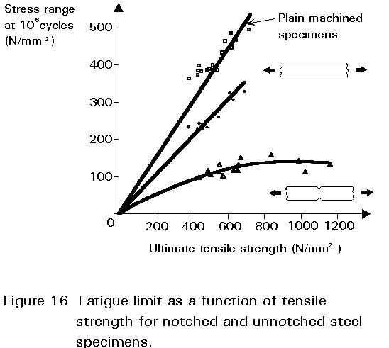
For real life components, the effects of notches, surface roughness and corrosion reduce the fatigue strength, the effects being strongest for the higher strength materials. The variation in fatigue strength with the tensile strength is illustrated in Figure 16. The data in Figure 16 are consistent with the fact that cracks are quickly initiated in components that are sharply notched or subjected to severe corrosion. The fatigue life then consists almost entirely of crack growth. Crack growth is very little influenced by the static strength of the material, as illustrated in Figure 16, and the fatigue lives of sharply notched parts are therefore almost independent of the tensile strength. An important example is welded joints which always contain small crack-like defects from which crack start growing after a very short initiation period. Consequently the fatigue design stresses in current design rules for welded joints are independent of the ultimate tensile strength.
Crack Growth Data
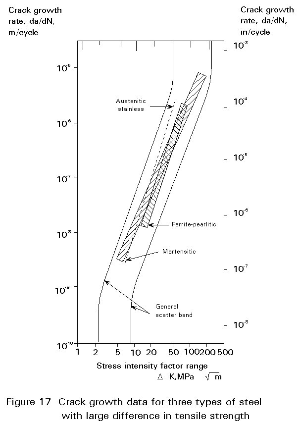
Fatigue crack growth rates seem to be much less dependent on static strength properties than crack initiation, at least within a given alloy system. In a comparison of crack growth data for many different types of steel, with yield strengths from 250 to about 2000 Mpa levels of steel, Barsom [4] found that grouping the steels according to microstructure would minimise scatter. His data for ferritic-pearlitic, matensitic and austenitic are shown in Figure 17. Also shown in the same diagram is a common scatter band which indicates a relatively small difference in crack growth behaviour between the three classes of steel. While data for aluminium alloys show a larger scatter than for steels, it is still possible to define a common scatter band. Recognising that different alloy systems seem to have their characteristic crack growth curves, attempts have been made to correlate crack growth data on the basis of the following expression
![]() = C
= C ![]() (3)
(3)
An implication of Equation 3 is that at equal crack growth rates, a crack in a steel plate can sustain three times higher stress than the same crack in an aluminium plate. Thus, a rough assessment of the fatigue strength of an aluminium component whose life is dominated by crack growth can be obtained by dividing the fatigue strength of a similarly shaped steel component by three.
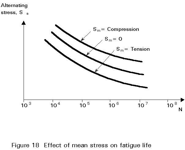
In 1870 Wöhler identified the stress amplitude as the primary loading variable in fatigue testing; however, the static or mean stress also affects fatigue life as shown schematically in Figure 10. In general, a tensile mean stress reduces fatigue life while a compressive mean stress increases life. Mean stress effects are presented either by the mean stress itself as a parameter or the stress ratio, R. Although the two are interrelated through:
Sm = Sa ![]() (4)
(4)
the effects on life are not the same, ie. testing with a constant value of R does not have the same effect on life as a constant value of Sm, the difference is shown schematically in Figure 18.
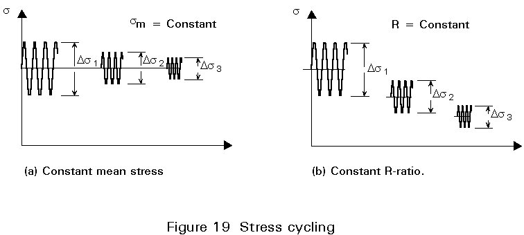
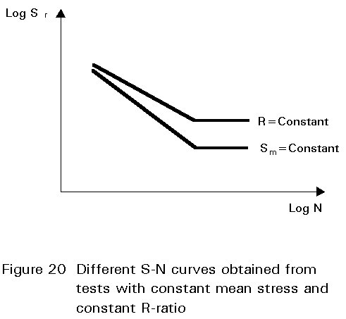
As indicated in Figure 19a, testing at a constant R value means that the mean stress decreases when the stress range is reduced, therefore testing at R = constant gives a better S-N curve than the Sm = constant curve, as indicated in Figure 19b. It should also be noted that when the same data set is plotted in an S-N diagram with R = constant or with Sm = constant the two S-N curves appear to be different, as shown in Figure 20.
The effect of mean stress on the fatigue strength is commonly presented in Haigh diagrams as shown in Figure 21, where Sa / So is plotted against Sm / Su. So is the fatigue strength at a given life under fully reversed (Sm = 0,R = -1) conditions. Su is the ultimate tensile strength. The data points thus represent combinations of Sa and Sm giving that life. The results were obtained for small unnotched specimens, tested at various tensile mean stresses. The straight lines are the modified Goodman and the Soderberg lines, and the curved line is the Gerber parabola. These are empirical relationships that are represented by the following equations:
Modified Goodman Sa/So + Sm/Su = 1 (5)
Gerber Sa/ So + (Sm/ Su)2 = 1 (6)
Soderberg Sa/ So + Sm/ Sy = 1 (7)
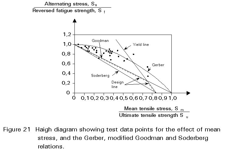
The Gerber curves gives a reasonably good fit to the data, but some points fall below the line, ie. on the unsafe side. The Goodman line represents a lower of the data, while the Soderberg line is a relatively conservative lower bound that is sometimes used in design. These expressions should be used with care in design of actual components since the effects of notches, surface condition, size and environment are not accounted for. Also stress interaction effect due to mean load variation during spectrum loading might modify the mean stress effects given in the three equations.
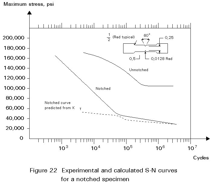
Fatigue is a weakest link process which depends on the local stress in a small area. While the higher strain at a notch makes no significant contribution to the overall deformation, cracks may start growing here and eventually result in fracture of the part. It is therefore necessary to calculate the local stress and relate this to the fatigue behaviour of the notched component. A first approximation is to use the S-N curve for unnotched specimens and reduce the stress by the Kt factor. An example of this approach is shown in Figure 22 for a sharply notched steel specimen. The predicted curve fits reasonably well in the high cycle region, but at shorter lives the calculated curve is far too conservative. The tendency shown in Figure 22 is in fact a general one, namely that the actual strength reduction in fatigues is less than that predicted by the stress concentration factor. Instead the fatigue notch factor Kf is used to evaluate the effect of notches in fatigue. Kf is defined as the unnotched to notched fatigue strength, obtained in fatigue tests:
Kf = ![]() (8)
(8)
From Figure 22 it is evident that Kf varies with fatigue life, however, Kf is commonly defined as the ratio between the fatigue limits. With this definition Kf is less than Kt, the stress increase due to the notch is therefore not fully effective in fatigue. The difference between Kf and Kt arise from several sources. Firstly, the material in the notch may be subject to cyclic softening during fatigue loading and the local stress is reduced. Secondly, the material in the small region at the bottom of the notch experiences a support effect caused by the constraint from the surrounding material so that the average strain in the critical region is less than that indicated by the elastic stress concentration factor. Finally, there is a statistical variability effect arising from the fact that the highly stressed region at the notch root is small, so there is a smaller probability of finding a weak spot.
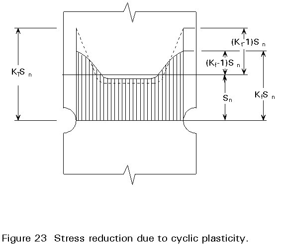
The notch sensitivity q is a measure of how the material in the notch responds to fatigue cycling, ie. how Kf is related to Kt. q is defined as the ratio of effective stress increase in fatigue due to the notch, to the theoretical stress increase given by the elastic stress concentration factor. Thus, with reference to Figure 21
q = (smax,eff - sn)/(smax - sn) = (Kfsn - sn)/(Ktsn - sn) = (Kf - 1)/(Kt - 1) (9)
where smax,eff is the effective maximum stress, see Figure 23. This definition of Kf provides a scale for q that ranges from zero to unity. When q = 0, Kf = Kt = 1 and the material is fully insensitive to notches, ie. a notch does not lower the fatigue strength. For extremely ductile, low strength materials such as annealed copper, q approaches 0. Also materials with large defects, eg. grey cast iron with graphite flakes have values of q close to 0. Hard brittle materials have values of q close to unity. In general q is found to be a function of both material and the notch root radius. The concept of notch sensitivity therefore also incorporates a notch size effect.
The fatigue notch factor applies to the high cycle range, at shorter lives Kf approaches unity as the S-N curves for notched and unnotched specimens converge and coincide at N = 1/4 (tensile test). In experimental investigations involving ductile materials it was found that the fatigue notch factor need to be applied only to the alternating part of the stress cycle and not to the mean stress. For brittle materials, however, Kf should be applied to the mean stress as well.
Although a size effect is implicit in the fatigue notch factor approach, a size reduction factor is normally employed in when designing against fatigue. The need for this additional size correlation arises from the fact that the notch size effect saturates at notch root radii larger than about 3-4mm, ie. Kf ® Kt, while it is well known from tests on full scale components, also unnotched ones, that the fatigue strength continues to drop off with increasing size, without any apparent limit.
The size effect in fatigue is generally ascribed to the following sources:
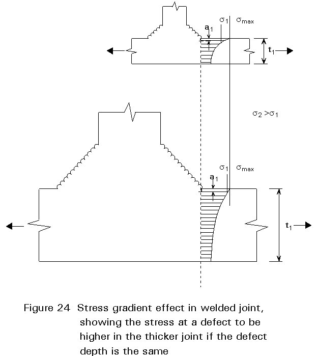
Examples of components for which the latter effect is important are welded joints and threaded fasteners. The critical locations for crack initiation are the weld toe and the thread root, respectively. In both cases the local stress is a function of the ratio of thickness (diameter) to the notch radius. In welds the toe radius is determined by the welding process and is therefore essentially constant for different size joints. The t/r ratio therefore increases and also the local stress when the plate is made thicker, with r remaining constant. A similar situation exists for bolts, due to the fact that the thread root radius is scaled to the thread pitch, rather than the diameter for standard (eg. ISO) threads. Since the pitch increases much slower than the diameter the result is an increase in the notch stress with bolt size. For bolts as well as welded joints the increased notch acuity effect comes in addition to the notch size effect discussed earlier, the result is that the experimentally determined size effects for these components are among the strongest recorded. An example of size effects for welded joints is shown in Figure 25. The solid line represents current design practice, according to eg. Eurocode 3 and the UK Department of Energy Guidance Notes. The equation for this line is given by:
![]() =
= ![]() (10)
(10)
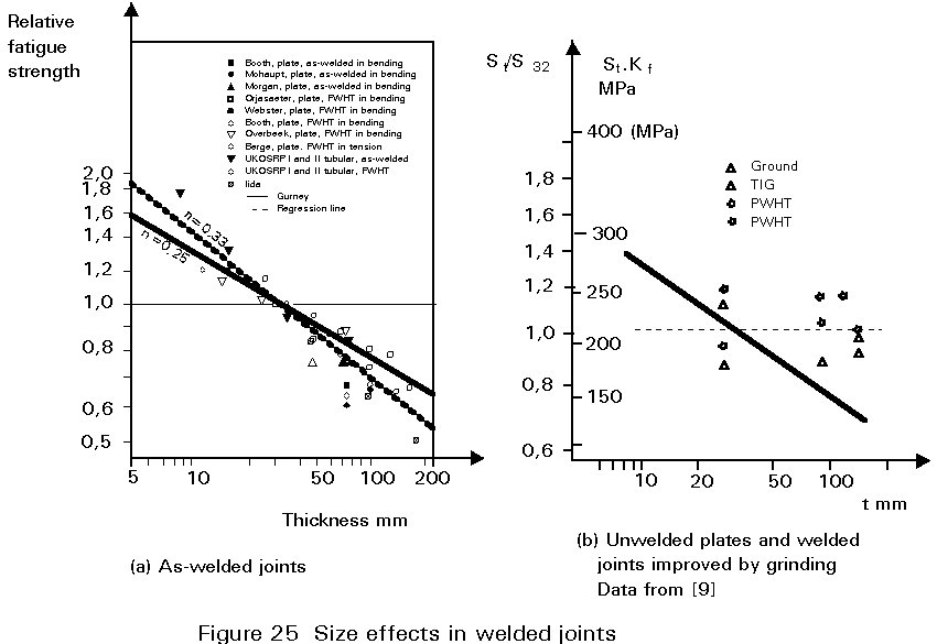
The exponent n, the slope of the lines in Figure 25a, is the size correction exponent.
The experimental data points indicate that the thickness correction with n = 1/4 is on the unsafe side in some cases. As indicated in Figure 25a thickness correction exponent of n = 1/3 instead of the current value of 1/4 gives a better fit to the data in Figure 25a. For unwelded plates and low stress concentration joints in Figure 25b a value of n = 1/5 seems appropriate [7].
There is experimental evidence that indicate a relationship between the stress gradient and the size effect. Based on an analysis of experimental data similar the following size reduction factor has been proposed to account for the larger stress gradient found in notched specimens [8].
n = 0.10 + 0.15 log Kt (11)
Almost all fatigue cracks nucleate at the surface since slip occurs easier here than in the interior. Additionally, simple fracture mechanics considerations show that surface defects and notches are much more damaging than internal defects of similar size. The physical condition and stress situation at the surface is therefore of prime importance for the fatigue performance. One of the important variables influencing the fatigue strength, the surface finish, commonly characterised by Ru, the average surface roughness which is the mean distance between peaks and troughs over a specified measuring distance. The effect of surface finish is determined by comparing the fatigue limit of specimens with a given surface finish with the fatigue limit of highly polished standard specimens. The surface reduction factor Cr is the defined as the ratio between the two fatigue limits. Since steels become increasingly more notch sensitive with higher strength, the surface factor Cr decreases with increasing tensile strength, Su.
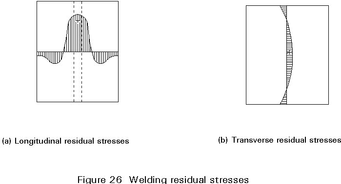
Residual stresses or internal stresses are produced when a region of a part is strained beyond the elastic limit while other regions are elastically deformed. When the force or deformation causing the deformation are removed, the elastically deformed material springs back and impose residual stresses in the plastically deformed material. Yielding can be caused by thermal expansion as well as by external force. The residual stresses are of the opposite sign to the initially applied stress. Therefore, if a notched member is loaded in tension until yielding occurs, the notch root will experience a compressive stress after unloading. Welding stresses which are locked in when the weld metal contracts during cooling are an example of highly damaging stresses that cannot be avoided during fabrication. These stresses are of yield stress magnitude and tensile and compressive stresses must always balance each other, as indicated in Figure 26. The high tensile welding stresses contribute to a large extent to the poor fatigue performance of welded joints.
Stresses can be introduced by mechanical methods, for example by simply loading the part the same way service loading acts until local plastic deformation occurs. Local surface deformation a such as shot peening or rolling are other mechanical methods frequently used in industrial applications. Cold rolling is the preferred method to improve the fatigue strength by axi-symmetric parts such as axles and crankshafts. Bolt threads formed by rolling are much more resistant to fatigue loading than cut threads. Shot peening and hammer peening have been shown to be highly effective methods for increasing the fatigue strength of welded joints.
Thermal processes produce a hardened surface layer with a high compressive stress, often of yield stress magnitude. The high hardness also produces a wear resistant surface; in many cases this may be the primary reason for performing the hardness treatment. Surface hardening can be accomplished by carburising, nitriding or induction hardening.
Since the magnitude of internal stresses is related to the yield stress their effect on fatigue performance is stronger the higher strength of the material. Improving the fatigue life of components or structures by introducing residual stresses is therefore normally only cost effective for higher strength materials.
Residual stresses have a similar influence on fatigue life as externally imposed mean stresses, ie. a tensile stress reduces fatigue life while a compressive stress increases life. There is, however, an important difference which relates to the stability of residual stresses. While an externally imposed mean stress, eg. stress caused by dead weight always acts (as long as the load is present), residual stress may relax with time, especially if there are high peaks in the load spectrum that cause local yielding at stress concentrations.
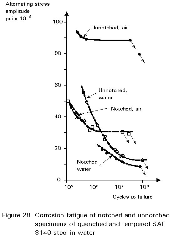
Corrosion in fresh or salt water can have a very detrimental effect on the fatigue strength of engineering materials. Even distilled water may reduce the high-cycle fatigue strength to less than two thirds of its value in dry air.
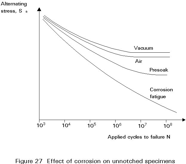
Figure 27 schematically shows typical S-N curves for the effect of corrosion on unnotched steel specimens. Precorrosion, prior to fatigue testing introduces notch-like pits that act as stress raisers. The synergistic nature of corrosion fatigue is illustrated in the figure by the drastic lower fatigue strength which is obtained when corrosion and fatigue cycling act simultaneously. The strongest effect of corrosion is observed for unnotched specimens, the fatigue strength reduction is much less for notched specimens, as shown in Figure 28.
Protection against corrosion can successfully be achieved by surface coatings, either by paint systems or through the use of metal coatings. Metal coating are deposited either by galvanic or electrolytic deposition or by spraying. The preferred method for marine structures, however, is cathodic protection which is obtained by the use of sacrificial anodes or, more infrequently, by impressed current. The use of cathodic protection normally restores the high cycle fatigue strength of welded structural steels to its in-air value, while at higher stresses hydrogen embrittlement effects may reduce the fatigue life by a factor of 3 to 4 on life.
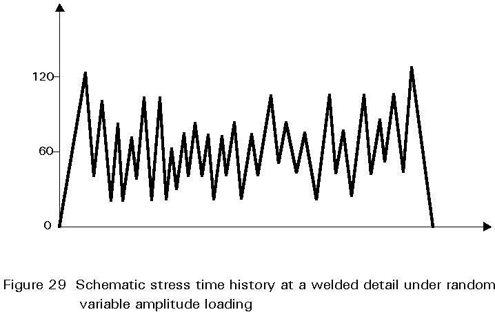
In practice the pattern of the stress history with time at any particular detail is likely to be irregular and may indeed be random. A more realistic pattern of loading would involve a sequence of loads of different magnitude producing a stress history perhaps as shown in Figure 29. The problem now arises as to what is meant by a cycle and what is the corresponding stress range. A number of alternative methods of stress cycle counting have been proposed to overcome this difficulty. The methods most commonly adopted for use in connection with Codes and Standards are the 'reservoir' or the 'rainflow' method.
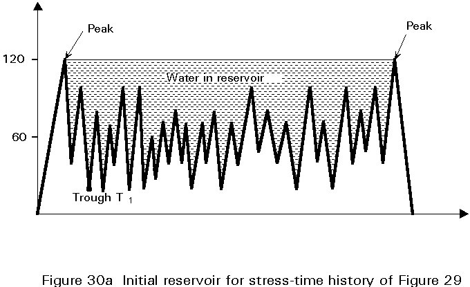
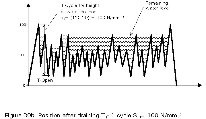
The basis of the reservoir method is shown in Figure 30 using the stress time history as Figure 29. it should be assumed that a stress time history of this kind has been obtained from strain gauges attached to the structure at the detail under consideration or has been estimated by computer simulation. It is important that the results analysed should be representative of long term behaviour. To analyse these results, a representative period is chosen so that the peak stress level repeats itself and a line is drawn to join the two peaks as shown in Figure 30a. The region between these two peaks is then regarded as being filled with water to form a reservoir. The procedure is then to take the lowest trough position and imaging that one opens a tap to drain the reservoir. Water drains out from this trough T1 but remains tapped in adjacent troughs separated by intermediate peaks as shown in Figure 30b. The draining of the first trough T1 corresponds to one cycle of stress range St as shown, and the remaining level of water is now lowered to the level of the next highest peak. A tap is now opened at the next lowest trough T2 as shown in Figure 30c and the water allowed to drain out. The height of the water released by this operation corresponds to one cycle of stress range S2. This procedure is continued sequentially through each next lowest trough, gradually building up a series of numbers of cycles of different stress ranges. It is also essential to allow for the one cycle from zero to peak stress. For the particular stress time history shown in Figure 29 the results obtained from the sample time period taken would be:
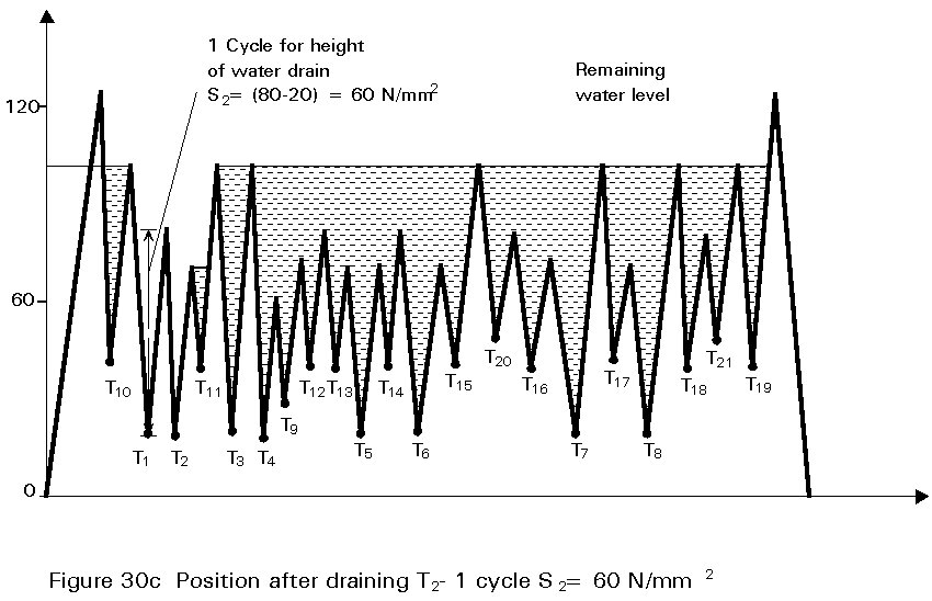
1 cycle at 120N/mm2, 1 at 100N/mm2, 4 at 80N/mm2, 6 at 60N/mm2, 10 at 30N/mm2.
The important principle of the above procedure is the recognition that by taking the difference between the lowest and highest stress levels (trough and peak) it is ensured that the greatest possible stress range is counted first, and this procedure is repeated sequentially so that the highest ranges are identified as the random fluctuations take place. In the assessment of the effects of the different cycles the greatest damage is caused by the higher stress ranges since the design curves follow a relationship of the kind SmN=constant. The reservoir method procedure does ensure that practical combinations of minima and maxima are considered together whereas this is not always the case in other stress cycle coating procedures.
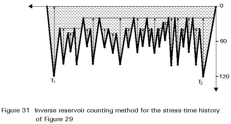
An alternative way of carrying out the reservoir cycle counting method is to turn the diagram upside down and use the complementary part of the diagram as shown in Figure 31. This version of the reservoir method gives identical results to the normal method but has the advantage of including the major cycle of stress from zero to maximum and back.
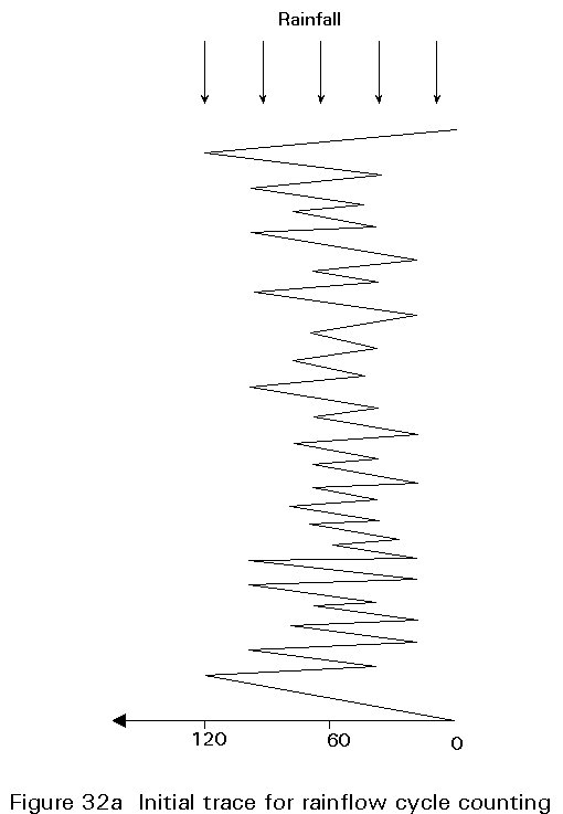
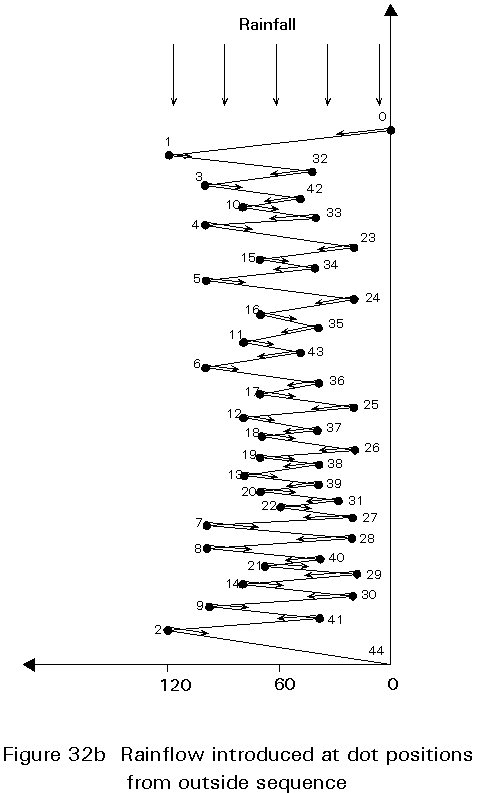
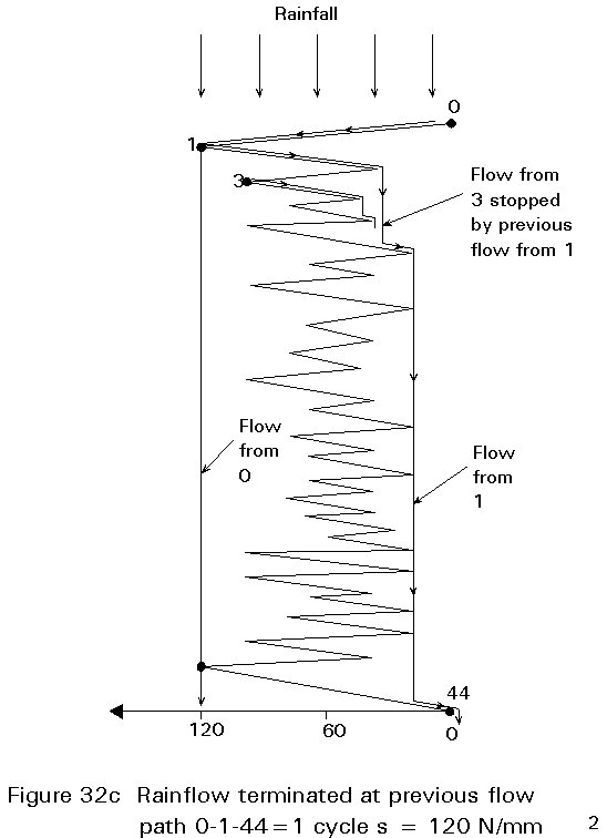
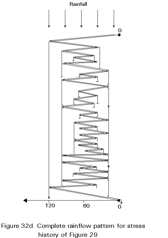
The alternative 'rainflow' cycle counting procedure is illustrated in Figure 32a for the same stress time history of Figure 29. This is essentially the same picture turned onto its side as shown in Figure 32a. Water (rain) is allowed to fall from the top onto the pattern considered as a roof structure and the paths followed by the rain are followed. However it is important that a number of standard rules are followed and the procedure is rather more complex and subject to error than the reservoir method. For each leg of the roof an imaginary flow of water is introduced at its highest point as shown by the dots in Figure 32b. The flow of water is followed for the outermost starting point first, allowing the water to drop onto any parts of the roof below and continue to drain until it falls off the roof completely. The width from the stress level at which the water started until it left the roof represents the magnitude of one cycle of stress. It is necessary to follow the flow paths from each starting point sequentially, moving progressively in from the points which are furthest out. If however the flow reaches a position where water has drained from a previous flow, it is terminated at that point as shown in Figure 32c for the flow starting from position 3 terminated by the previous flow position 1. The stress range for a cycle terminated in this way is limited to the width between the starting point and the termination point. The complete rainflow diagram for the stress pattern of Figure 29 is shown in Figure 32d. This procedure when correctly applied also counts the highest stress range cycles first and ensures that only practical combinations of minima and maxima within a sequence are considered. The rainflow method is somewhat more difficult to apply correctly than the reservoir method and it is recommended that both for teaching and for design purposes the reservoir method should be used. The results for the stress ranges from the rainflow method applied to the stress history from Figure 29 are identical to those from the reservoir method ie.
1 cycle at 120N/mm2, 1 at 100N/mm2, 4 at 80N/mm2, 6 at 60N/mm2, 10 at 30N/mm2.
There are two other cycle counting methods, the 'range pair counting' method and the 'mean crossing level' which are sometimes used although they tend not to be specified in Codes.
Example 1 This design example is based on the stress cycle history of Figure 29 as analysed above for stress cycle counting purposes. Firstly the stress history represents a relatively short time period, and has to be extrapolated to represent the total required life. Obviously the first requirement is to ascertain the required design life, and to multiply the numbers of cycles of each stress range determined as above by the ratio of the design life to the period represented by the sample time record taken. For example, if the design life was 20 years, and the sample time period was 6 hours, the numbers of cycles should be multiplied by 20 x 365 x 4 = 29200. Caution should be exercised with such an extrapolation however, as to whether such a short length time sample is representative of long term behaviour. For example in the case of a bridge structure the traffic flows are likely to vary at different times of day, peaking at rush hour times and falling to low values in the middle of the night. Furthermore there is possibility that the heaviest loads may not have occurred during the sampling time considered. Problems of extrapolation from samples to full data are common in the statistical world and statistical procedures may be necessary to ensure that potential differences in scaling up the data are allowed for. To a large extent this depends on the absolute size of the sample taken.
To check whether the design is satisfactory for any particular detail, it is necessary to decide on the appropriate design S-N design curve for the detail. The basis of doing this for Eurocode 3 will be explained in Lecture 12.9. For present purposes it will be assumed that the stress history of Figure 29 analysed above applies to a detail for which the design S-N curve is S90, for which the design life is 2 x 10⁶ cycles at stress range 90N/mm2 with slope - 1/3 continued down to a stress level of 66N/mm2 at design life 5 x 10⁶ cycles, with a change in slope to -1/5 on down to a stress range of 36N/mm2 which is the fatigue limit at 10 million cycles. For a twenty year design life assuming the stress history of Figure 29 is representative of 6 hours typical loading the following table can be constructed:
|
Stress range N/mm2 |
Cycles applied n |
Available cycles N |
n N |
|
120 |
29200 |
843750 |
0.0346 |
|
100 |
29200 |
1.458 x 10⁶ |
0.0200 |
|
80 |
116800 |
2.848 x 10⁶ |
0.0410 |
|
60 |
175200 |
8.053 x 10⁶ |
0.0218 |
|
30 |
292000 |
below cut off |
0 |
|
S n/N = |
0.1174 |
For these assumptions the loading is acceptable for the detail and life required. Indeed the 'Damage Sum' value of 0.1174 based on a 20 year design life indicates the available design life is 20/0.1174 = 170 years. For this particular case the stress range of 60N/mm2 fell in the intermediate range between 36 and 66N/mm2 and the available life N was calculated using the changed slope of the S-N curve for this region. The stress range of 30N/mm2 is below the cut off for the S90 classification and does not contribute to the fatigue damage.
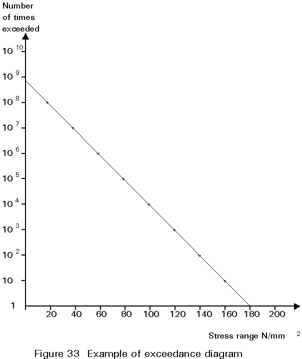
A convenient way of summarising the fatigue loading applied to structures is by the use of exceedance diagrams. These diagrams present a summary of the magnitude of a particular event against the number of times this magnitude is exceeded. Whilst in principle this presentation can be applied to a wide variety of phenomena for the purposes of fatigue analyses the appropriate form is a graph of log (number of times exceeded) against the occurrence of different stress levels. An example is shown in Figure 33. This might represent the stresses caused at a particular location in a bridge by traffic passing over r by wave loading of an offshore structure. A typical feature of natural phenomena of this kind is that the number of exceedances increases as the stress level decreases. The form of the exceedance diagram for natural phenomena of this kind is often close to linear as shown. It is important to note that the diagram represents exceedances so that any particular point on the graph includes all of the numbers of cycles of stress range above that value. For use in fatigue analysis using Miner's law the requirement is a summary of the numbers of cycles of each stress level occurring. Thus the loading represented by the exceedance diagram of Figure 33 can be treated as an equivalent histogram with cycles as follows:
|
Stress range N/mm2 |
No. of times exceeded |
Cycles occurring |
|
180 |
1 |
1 |
|
160 |
10 |
9 |
|
140 |
100 |
90 |
|
120 |
1000 |
900 |
|
100 |
10000 |
9000 |
|
80 |
100000 |
90000 |
|
60 |
1000000 |
900000 |
|
40 |
10000000 |
9000000 |
|
20 |
100000000 |
90000000 |
Some of the stress ranges will be found to be below the fatigue limit and hence will not contribute to the Miners law damage sum. For example for the detail considered in Example 1 above, the cut off limit was 36N/mm2 and the stress ranges of 20N/mm2 would not contribute to the fatigue damage. The stress ranges above this level will contribute however and their effects must be included. This is done by finding the value of S SmN separately for the remaining stress levels above and below the change in slope of the S-N curve, and for the figures given above this will be found to be 5.692 x 10¹⁰ for stress ranges of 80N/mm2 and above, and 1.621 x 10¹⁵ for the 40 and 60N/mm2 stress ranges. For an S90 detail with the spectrum of loading shown above, the fatigue damage from each part of the S-N curve has to be calculated based on the appropriate value of SmN=constant as follows:
![]() +
+ ![]() = 0.298
= 0.298
From these figures the damage sum factor calculated as 0.298 is acceptable. Detailed examination of the figures leading up to this result would indicate that the majority of the damage calculated occurs at the lowest stress ranges of 40 and 60N/mm2 contributing to the S5N part of the design curve.
Block loading is a particular case of an exceedance diagram.
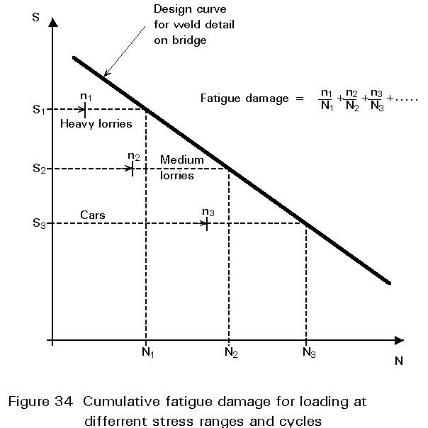
Consider the particular case of a one lane bridge structure on which the loading is idealised as falling into three categories. Suppose that there are n1 heavy lorries travelling across the bridge during its lifetime, and that at a particular welded detail each lorry causes a stress range S1. In addition there are n2 medium lorries which cause a stress range S2, and n3 cars which cause a stress range S3 at the same welded detail as they cross the bridge. To assess the combined effect of the different stress ranges all being applied in some form of sequence the procedure adopted is to assume that the damage caused by each individual group of cycles of a given stress range is the same as would be caused under constant amplitude loading at that stress range. It is necessary first to decide on the appropriate classification for the geometric detail being considered and to identify the appropriate S-N design curve. For present purposes, let us assume that the design curve is as shown in Figure 34. If the only fatigue loading applied to the bridge was the crossing of the heavy lorries with stress range S1 at the detail concerned, the available design life would be N1 cycles as shown in Figure 34. In fact the number of cycles applied at this stress range is n1. It is assumed that the fatigue damage caused at stress range St is n1/N1. Similarly if the only fatigue loading applied to the bridge was the crossing of the medium lorries with stress range S2 the available design life would be N2 and the fatigue damage caused would be n2/N2. For the passage of the cars at stress range S3 the available design life if this was the only loading would be N3 and the fatigue damage caused would be n3/N3. When all three loadings occur together the assumption for design purposes is that the total fatigue damage is the sum of that occurring at each individual stress range independently. This is known as the Palmgren-Miner law of linear damage, or more simply as Miner's law and is summarised as follows:
![]() +
+ ![]() +
+ ![]() + .... + = 1 (11)
+ .... + = 1 (11)
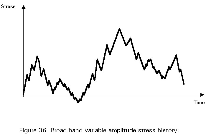
It is not uncommon for loading to occur at more than one frequency. It is generally considered that for non aggressive environmental conditions, eg. steel in air, there is little or no effect of frequency on constant amplitude fatigue behaviour. In aggressive conditions however, eg. steel in seawater, there may be significant effects of frequency on the crack growth mechanism leading to increased crack growth rates, shorter lives and reduction or elimination of the fatigue limit. In particular it is necessary in fatigue testing of materials where environmental conditions may be important to carry out the testing at the same frequency as that of the service loading. An example of this is the effect of wave loading on offshore structures where a typical frequency of waves is about 0.16Hz. Clearly this has major implications on the time required for testing since to accumulate one million cycles at 0.16Hz would take about 70 days whereas a conventional test in air at say 16Hz would reach the same life in less than 1 day. With any structure the response of the structure to dynamic loading depends on the frequency or rate of the applied loading and on the vibration characteristics of the structure itself. It is most important for the designer to ensure that the natural resonance frequencies of the structure are well separated from the frequencies of applied loading which may occur. Even so the structure may respond with frequencies of stress fluctuation which are a combination of the applied loading frequency and its own natural vibration frequencies. Furthermore since the magnitude of the loading may also vary with time it is necessary to consider both time domain and frequency domain aspects. Figure 35 shows a typical frequency domain response for stress fluctuations at a particular location in an offshore structure. This diagram gives information on number of times different stress levels are exceeded as well as the frequency data. The peaks at about 0.16Hz correspond to the applied loading whereas the higher frequency peaks are those due to the vibration response of the structure.
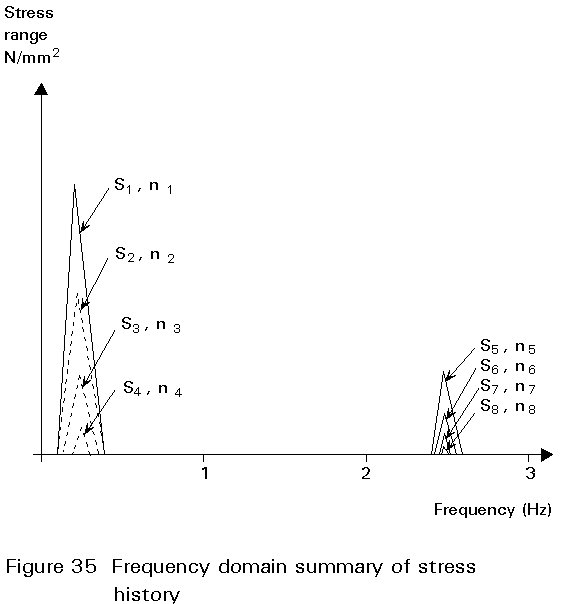
With variable amplitude fatigue loading of this kind there are additional complexities with regard to frequency effects to be considered. Where the stressing occurs close to or at a single frequency the condition is known as 'narrow band' and when there are a range of different frequencies involved it is known as 'broad band'. If the frequency domain response of Figure 35 is converted back into the time domain response in which the data was originally recorded the result would look like Figure 36. Clearly some assumptions must have been in the conversion of one diagram into the other and in this case it is that stress cycle counting has been carried out by the reservoir method. In Figure 36 however, it is clear that because the higher frequency stress cycles are superimposed on top of the lower frequency cycles, some of the higher frequency cycles occur at higher mean stress or stress ratio.