ESDEP WG 12
FATIGUE
To introduce the main concepts and derivation regarding both the statistical evaluation of the fatigue strength of structural details and the determination of partial safety coefficients on which are founded the fatigue assessment rules in Eurocode 3 [1].
None.
Lecture 12.8: Basic Fatigue Design Concepts in Eurocode 3
This lecture presents an overview of the statistical analysis procedure applied to fatigue test data of a particular detail in order to derive the most appropriate S-N curve. Special attention is given to the definition of the partial safety factors which are in Eurocode 3 for fatigue design assessment [1]. The use of a proper fatigue damage-tolerant level is discussed which is based on sufficient residual strength and stiffness in remaining members between inspection intervals until the fatigue crack can be detected and repaired.
Fatigue failure may arise in many engineering structures submitted to repeated loadings. Many failures occurring in structures are due to the process of fatigue crack propagation. Fracture may be in encountered in many civil engineering structures such as bridges, cranes, gantry girders, offshore or marine structures, transmission towers, chimneys, ski lifts, etc. The safe-life prediction of structures subjected to fatigue loading is recognised as being a very difficult problem. The stresses in any civil engineering structure are often caused by random loading; the properties of the materials, and the fabrication conditions for the structure may also vary in a random manner. The integrated influence of all these variables yields a wide scatter in life prediction.
As a result, in spite of the progress made in the understanding of the fatigue mechanism, and of the conservatism introduced in design against fatigue failure, design rules are still based on a "damage-tolerant approach" which is more or less substantiated by reliability analyses.
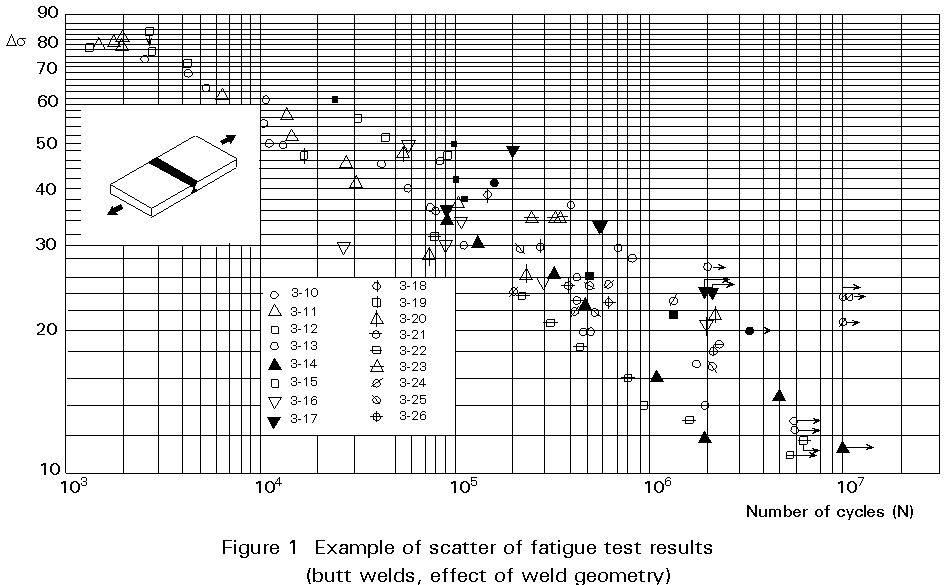
The S-N curves are evaluated from a series of fatigue tests performed on specimens which comprise the structural detail for which assessment of the fatigue strength is required. When the fatigue test results are plotted on a log-log scale, i.e. log (stress range, Ds ) versus log (number of cycles to failure) a considerable statistical scatter exists in the fatigue data as illustrated in Figure 1.
Instead of taking a lower bound limit approach, a statistical evaluation of the fatigue test results is performed. Assuming a linear relationship between log Ds and log N the following equation may be written:
log N = log A - m . log Ds (1.1)
Let
y = log N; x = log Ds ; a = log A; b = - m (1.2)
where log is the logarithm to base 10.
The first step of the statistical analysis is to apply a technique of standard linear regression analysis of the data to find estimates of a and b, denoted
![]() and
and ![]() respectively. Each pair of fatigue data, yi = log Ni and xi = log Dsi, should satisfy the relation:
respectively. Each pair of fatigue data, yi = log Ni and xi = log Dsi, should satisfy the relation:
yi = ![]() +
+ ![]() . xi + ei (1.3)
. xi + ei (1.3)
where ei is called the residual.
The estimates ![]() and
and ![]() are determined so that the sum of the squares of the residuals is a minimum. This condition leads to the following estimates [2].
are determined so that the sum of the squares of the residuals is a minimum. This condition leads to the following estimates [2].
![]() =
=  (1.4)
(1.4)
and
![]() =
= ![]() =
= ![]() .
. ![]() (1.5)
(1.5)
where ![]() and
and ![]() are respectively the means of yi and xi, i.e.
are respectively the means of yi and xi, i.e.
![]() =
= ![]() ,
,
![]() =
= ![]() where n is the number of data points (sample size).
where n is the number of data points (sample size).
The second step is to find the variance of the distribution f(yi) at a given xi. The variance of yi, written Var(yi), is assumed to be constant for all values of xi=logDsi. The constant variance assumption is sometimes questionable, but holds true for a majority of fatigue test data. It is also usually assumed that, for any fixed value of xi, the corresponding value of yi forms a normal distribution.
One of the main comparison indicators which is used in relation to the classification system adopted in Eurocode 3 [1] is the characteristic strength at two million cycles, written xc = log Dsc. Let yc = log Nc be the random variable corresponding to a given value xc.
The sampling distribution of yc may be obtained from the following estimation [2]:
![]() c =
c = ![]() +
+ ![]() .xc (1.6)
.xc (1.6)
and
![]() (1.7)
(1.7)
where Var (yc/xc) is the variance of yc given that x is equal to xc.
![]() (1.8)
(1.8)
where
![]() (1.9)
(1.9)
A 95% confidence interval estimate for yc is given by:
![]() (10)
(10)
where t95 is the 95% percentile of the Student's distribution with n-2 degrees of freedom [2]. Thus there is confidence that 95% of the yc Student's t population will have values above yck.
Very often in fatigue test analysis the sample size is small (n£ 30) and the value of the estimation of the variance of yc as defined by Equation (1.7) fluctuates considerably from sample to sample. To take this fact into account, the distribution of f(yi) for sample size n £ 30 has been assumed to follow a Student's t distribution.
Knowing yck from Equation (1.10), the characteristic strength at two million cycles may be calculated from Equation (1.1). Finally the "one-sided" confidence estimate is performed for a particular point referred to as the characteristic strength at two million cycles.
The characteristic S-N curve is given by the following equation:
log Nk = (log A - t95sycxc) - m.log Dsk (1.11)
and the characteristic strength at two million cycles may be calculated from:
log Dskc = [(log A - t95sycxc) - log (2 × 10⁶)]/m (1.12)
Therefore
Dskc =10logDskc (1.13)
Numerical Example
Assume a given detail has been tested under constant amplitude fatigue loading. The fatigue test data is reported in the following Table. No failure was observed for the first five specimens for a number of cycles over two million. The characteristic fatigue strength curve corresponding to the given detail is determined as follows:
|
Stress Range Ds (N/mm²) |
Number of Cycles N (x 1000) |
Failure Identification |
|
74 74 108 108 108 108 108 139 139 202 202 202 265 265 265 |
Over 2000 id id id id 1077 800 597 537 204 188 107 79 70 42 |
not failed not failed not failed not failed not failed failed id id id id id id id id id |
Table Fatigue Test Data
First Step: Perform the linear regression analysis:
The evaluation of a and b according to Equations (1.4) and (1.5) may be obtained from the following numerical Table which includes only the tests that have resulted in a fatigue failure.
|
No |
D s i (N/mm²) |
xi=log D s i |
yi=log Ni |
x21 |
y21 |
x1.y1 |
|
1 2 3 4 5 6 7 8 9 10 |
108 108 139 139 202 202 202 265 265 265 |
2,03 2,03 2,14 2,14 2,31 2,31 2,31 2,42 2,42 2,42 |
6,032 5,903 5,776 5,730 5,310 5,274 5,029 4,898 4,845 4,623 |
4,135 4,135 4,593 4,593 5,315 5,315 5,315 5,872 5,872 5,872 |
36,388 34,846 33,362 32,833 28,192 27,817 25,295 23,987 23,475 21,374 |
12,266 12,003 12,378 12,279 12,241 12,159 11,594 11,868 11,741 11,203 |
|
S |
22,5387 |
53,4204 |
51,0149 |
287,568 |
119,733 |
b = ![]()
a = ![]()
therefore, the linear regression equation is given by:
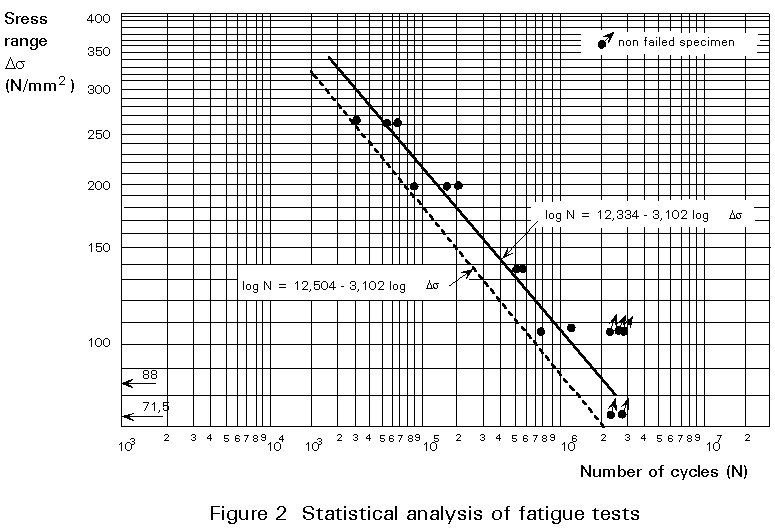
log N = 12,334 - 3,102 log Ds (1.11)
for Nc = 2000 000 cycles, from (1.11):
log Dsc = 1,945 and Dsc = 88,05 N/mm2
Second Step: To find the variance of y = log N
from the calculation table above.
![]()
![]()
![]()
![]()
and the variance:

The standard deviation is then
s
yc/xc = 0,151The Student's t95 value with n - 2 = 8 degrees of freedom can be obtained from a statistical table of the t distribution [3]:
t95 = 1,860
The characteristic strength at two million cycles is then:
log Dskc = ![]()
Therefore:
Dskc = 101,854 = 71,5
In conclusion, referring to the basic S-N curves in Eurocode 3 (Fig. 9.6.1 in Eurocode 3), the detail analysed under the preceding statistical evaluation may be classified under category 71, Figure 2.
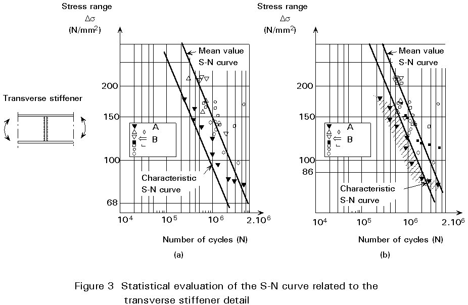
The standard deviations vary from test to test and from the type of detail studied. In general, the higher the stress concentration factor, the lower the standard deviation of the fatigue test results. The following table gives some indication of the standard deviations which were obtained when performing the statistical analysis of various types of detail category. When mixing fatigue test results from various sources, the standard deviation tends to increase and care should always be exercised to minimise problems arising from inhomogeneity of data, Figure 3. These values of the standard deviation of the number of cycles given in the table are somewhat different to the values appearing in Annex C of reference [4] due to the fact that more complete sources of fatigue data where analysed when reviewing the classification for Eurocode 3 [5].
|
Type of detail |
Range of standard deviation s yc/xc |
|
Rolled beam Welded beam Vertical stiffener Transverse attachment Longitudinal attachment Cover plate on flange Bolted connection in shear |
0,125 - 0,315 0,150 - 0,230 0,115 - 0,170 0,115 - 0,190 0,110 - 0,140 0,070 - 0,140 0,230 |
A structural element submitted to fatigue loading is subjected to several uncertainties. The variability of the parameters governing the fatigue life of a structural element, i.e. fatigue loading and fatigue resistance are largely unknown. A level II reliability model has been implemented for the derivation of recommended partial safety factors in relation to the following fatigue strength assessment equation:
g
f Dss = DsR/gM (3.1)where
Ds
s is the equivalent constant applied stress range which, for the given number of cycles, leads to the same cumulative damage as the design spectrum.Ds
R is the fatigue strength as given by the S-N curve of the relevant detail category.g
f and gM are the partial safety factors applied respectively to the spectrum loading and to the resistance.It will be assumed that log Dss and log DsR are both random variables following a normal distribution law. Therefore the random variables Dss and DsR are said to follow a log-normal distribution.
The fatigue limit state function may be written as:
g = log DsR - log Dss (3.2)
Introducing the normalised basic variables u and v as:
u = {log DsR - ![]() }
/ SlogDsR (3.3)
}
/ SlogDsR (3.3)
v = {log DsS - ![]() }
/ SlogDsS
}
/ SlogDsS
![]() is the mean value and SlogDsR is the standard deviation of the variable log DsR.
is the mean value and SlogDsR is the standard deviation of the variable log DsR.
The limit state function, Equation (3.2), re-written with the normalised basic variables becomes:
g(u,v) = SlogDsR.u - SlogDsS.v
+ ![]() -
- ![]() (3.4)
(3.4)
Having assumed that the random variables log DsS and log DsR are normally distributed, then the safety index b is related to the probability of failure P as:
P
= F(-b) (3.5)in which F(-b) is the standardised normal distribution function and b is given by (it is assumed for the sake of simplicity that the variables u and v are uncorrelated):
b
= {It is recalled that b can be geometrically interpreted as the shortest distance from the origin to the failure surface in the standard normal space, Figure 4.
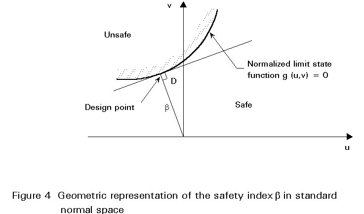
The coordinates of the design point D represent the values of u and v with the highest probability of failure. These coordinates are expressed by:
a
u = -bSlogDsR / Ö(S2logDsR + S2logDsS) (3.7)a
v = b SlogDsS / Ö(S2logDsR + S2logDsS)Rearranging Equation (3.7) in terms of the basic variables log DsS and log DsR gives:
a
R =a
s =The characteristic values of the random variables (log DsRk and log Dssk) are then expressed by:
log DsRk = (log DsR)k
= ![]() (1 - kR CR)
(3.9)
(1 - kR CR)
(3.9)
log Dssk = (log Dss)k
= ![]() (1 + ks Cs)
(1 + ks Cs)
where Cs and CR are respectively the coefficients of variation of log Dss and log DsR (i.e. the ratio of standard deviation over the mean value).
To determine the partial safety factors in a semi-probabilistic format (level I reliability format), which corresponds to the same degree of safety (represented by the safety index b) as a level II reliability format, one has to utilize the Equations (3.8) and (3.9). Assuming:
m
= Slog DsR/Slog DsRthen the partial factors can be obtained from the following relations:
log gM = Slog DsR b /[Ö(1+ m2)] - kR (3.10)
log gf = mSlog Dss bm /[Ö(1+ m2)] - ks
For a defined safety index b the partial safety coefficients may be calculated from Equations (3.10), knowing the standard deviations of the resistance and the loading (Slog DsR and Slog Dss) and the coefficients kR and kS related to the definition of the characteristic values adopted for (log DsR)k and (log Dss)k.
Remarks
Slog Dss = log e Ö[ln(1 + Vs2)] (3.11)
with by definition:
Vs = SDss / ![]()
where e is the Euler's number and ln is the Naperian logarithm.
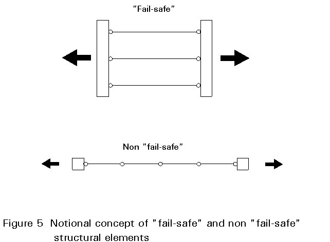
It must be understood that the safety indices which were proposed (see Table 1) in Eurocode 3 (Chapter 9) are mainly based on an engineering judgement of what may be called a potential risk of acceptance of losses and damages. It is the responsibility of each concerned authority to make the decision on the proper choice of these values on the basis of a realistic risk assessment.
|
"Fail-Safe" structural detail |
"Non fail-safe" structural detail |
|
|
Periodic inspection and maintenance. Accessible joint detail. |
b = 2 |
b = 3 |
|
Periodic inspection and maintenance. Poor accessibility. |
b = 2,5 |
b = 3,5 |
Table 1 Recommended values of safety indices
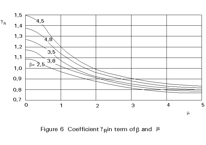
Figure 6 gives the partial safety coefficient gR in terms of b and m. These curves have been drawn for kR=2 and kS=1,645 and for slogDsR=0,07 (which corresponds to slogN=0,210.
In Chapter 9 of Eurocode 3 [1] values of the product gf.gM have been proposed (Table 2) based on the values of safety indices given in Table 1. There is little information concerning fatigue loadings and if the partial safety factor gf is known, then the partial safety factor gM related to the strength must be adjusted.
|
"Fail-safe" structural detail |
"Non fail-safe" structural detail |
|
|
Periodic inspection and maintenance. Accessible joint detail. |
g = 1,00 |
g = 1,25 |
|
Periodic inspection and maintenance. Poor accessibility. |
g = 1,15 |
g = 1,35 |
Table 2 Recommended values of the product g = gf.gM
Remarks
Discontinuities play a major role in the fatigue strength, particularly for welded details. Careful consideration must be given to the weld quality since it significantly affects fatigue strength variation. Moreover, the measures that can be taken to achieve the required degree of structural reliability include not only the justification of relevant design rules and the choice of associated partial safety factors, but also an appropriate level of execution quality and proper standards for workmanship which are developed in pr EN 1090-1 [6].
(i) The structure must have an adequate life either crack-free or during which the growth rate of cracks is sufficiently low to allow detection during an inspection period.
(ii) Visual inspection of all critical areas is possible in service.
[1] Eurocode 3: "Design of Steel Structures": ENV 1993-1-1: Part 1.1, General Rules and Rules for Buildings, CEN, 1992.
[2] Walpole E.R. and Myers R.H., Probability and statistics for engineers and scientists, MacMillan Publishing Co. Inc., New York, 2nd Ed., 1978
[3] Natrella M.G., Experimental Statistics, National Bureau of Standards Handbook 91, Issued August 1 1963. Reprinted October 1966 with corrections.
[4] Recommendations pour la vrification la fatigue des structures en acier. CECM - Comit Technique no. 6: "Fatigue". CECM no. 43, 1987, Premire dition.
[5] Background Documentation to Eurocode 3: Chapter 9 - Fatigue, Background information on fatigue design rules: Statistical Evaluation, December 1989.
[6] prEN 1090-1:1993 Execution of steel structures, Part 1: General rules and rules for buildings.