ESDEP WG 12
FATIGUE
This lecture gives an introduction to the methods of analysis of cracked bodies and reviews the main concepts of fracture mechanics. These concepts are necessary to understand the design considerations for fracture assessment under static loading and fatigue under repeated loading as specified in Annex C and Chapter 9 of Eurocode 3, [1].
An understanding of plasticity [2,3].
Lecture 12.10: Basics of Fracture Mechanics
Lecture 12.12: Determination of Stress Intensity Factors
Lecture 12.14: Fracture Mechanics Structural Engineering Applications
Lecture 12.15: Fracture Mechanics Applied to Fitness for Purpose
The lecture begins by outlining the primary basis, within the framework of linear-elastic fracture mechanics, for determining the stress field in the local region ahead of a crack tip embedded in a solid body. Then, it briefly discusses models used to assess the local plastic zone existing in front of the crack tip.
All structural elements have discontinuities, either created unintentionally during fabrication or developed during service conditions under repeated load to which the structure is subjected. Discontinuities will affect the strength of a structural element and may lead to fracture under a particular state of stress induced by static or fatigue loading.
Various fracture mechanic quantities have been introduced to give a measure of the severity of an existing crack in a body, e.g. the stress intensity factor K, the Rice's J integral, the energy release rate G (which is the amount of energy released during an incremental increase of the crack area) the crack opening displacement COD. All these quantities are related to one another under specific assumptions. The most used of these quantities, which characterize the local stress and strain field in the vicinity of a crack is the stress intensity factor K. This parameter, fundamentally derived from linear elastic fracture mechanics, is a function of the applied stress and the geometrical configuration and dimensions of both the crack and the body which contains the crack.
This lecture is an introductory lecture to the two main applications of fracture mechanics, which will be developed in subsequent lectures. The first application is the design against fracture of cracked elements subjected to particular temperature and loading conditions. The safe design is achieved when the stress intensity factor K is less than a critical value Kc known as the fracture toughness. The second and more common application is related to fatigue crack growth conditions under repeated loading cycles. It is proved experimentally that, for steel structural material, the rate of crack propagation is a function of the range of stress intensity factor. Slow stable crack propagation which mainly governs the fatigue life of welded structural elements takes place for values of K smaller than a critical value Kd somewhat different from the previously defined fracture toughness Kc.
Having in mind these two applications this lecture is mainly concerned with linear fracture mechanic concepts. The analytical basis in assessing local stress field near the flaw is described, and then some considerations concerning plasticity at the crack tip are introduced. Finally, approximate methods for the evaluation of stress intensity factors in more general cases are given.
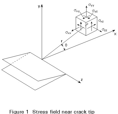
The stresses and strains at any point near a crack tip (Figure 1) can be derived from the theory of elasticity. Stresses and strains within the interior of a solid body subjected to external load and/or displacement conditions are known to satisfy a set of fundamental differential equations resulting from equilibrium, compatibility conditions and physical properties of the material which constitutes the solid body.
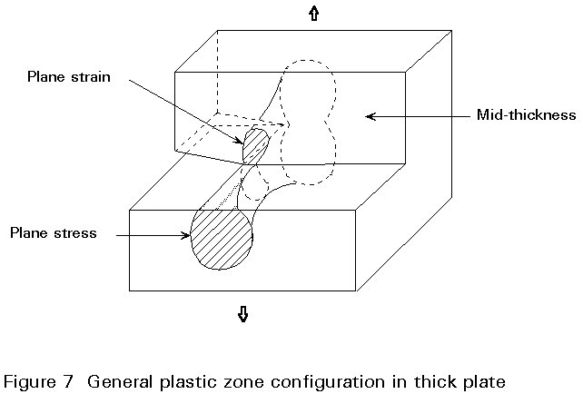
The process of solution of a problem of plane elasticity consists of finding a particular mathematical function of the distribution of stresses (or strains) which fulfils not only these differential equations, but also satisfies the boundary conditions expressed in term of forces or displacements specified over the surface of the body. In plane stress problems (i.e. szz = szx = szy = 0; which is the case of thin plates) or plane strain problems (i.e. exz = eyz = ezz = 0; which corresponds to the condition of strains existing at mid-thickness of a thick plate) the usual method of solving the set of differential equations is to introduce the so-called Airy stress function.
The solution of a plane elasticity problem is reduced to finding a biharmonic function F satisfying the conditions expressed previously. It can be demonstrated [4] that, for zero body forces, the stresses may be derived in the plane elasticity problem from the following relations:
s
xx = ¶2F/¶y2s
yy = ¶2F/¶x2 (2.1)s
xy = ¶2F/¶x¶yFor discontinuous boundary conditions, the classical polynomial method is not suitable if boundary conditions are to be precisely satisfied. Westergaard and Mushkelishvili have developed independently general methods for stress function solutions which are well suited to solve plane problem of elasticity for cracked body. The Westergaard method is more particularly applicable to crack problems in infinite plate.
The method proposed by Westergaard [5] systematically expresses the Airy stress function F in terms of general harmonic functions to a desirable form:
F = f1 + x.f2 + y.f3 (2.2)
where
F is biharmonic when f1, f2, and f3 are harmonic functions.
Westergaard chooses the functions f1, f2, or f3 as the real and imaginary parts of an analytical function and its derivatives (named the Z functions). Taking into account the particularity of the problem, such as the symmetry of the stress field, F can be simplified by taking f2 or f3 = 0. Assuming Z as the analytical function, its derivatives are:
Z¢ = dZ/dz; Z² = dZ¢ /dz; Z'" = dZ² /dz (2.3)
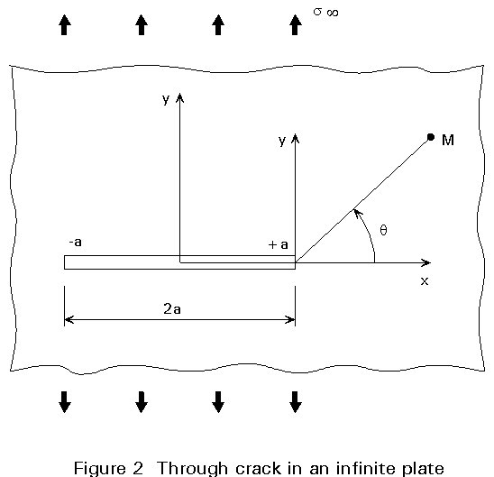
If there is a displacement continuity in the y axis direction (Figure 2) and a crack parallel to the x direction, due to symmetry of the stress field, the Airy stress function as expressed by Equation (2.2) may be written:
F = Re Z + y . Im Z¢ (2.4)
Re and Im are respectively the real and imaginary parts of the Z functions. The polar coordinate r and q (Figure 2) are used to locate any point in the local region ahead of the crack tip, therefore
z = ieiq = x + iy
From Equation (2.4) following expressions are derived:
2F/¶x2 = Re Z" + y . Im Z'"
2F/¶y2 = Re Z" - y . Im Z'" (2.5)
2F/¶x¶y = y . Re Z"Therefore, taking into account Equations (2.5), the stresses as given by Equation (2.1) are expressed by:
s
xx = Re Z" - y . Im Z'"s
yy = Re Z" + y . Im Z'" (2.6)s
xy = - y . Re Z"It can be seen, that this type of Airy stress function satisfies certain problems for which symmetry conditions hold, e.g. for y = 0; sxx = syy and sxy = 0.
The Z functions, must fulfil the boundary conditions of the problem. The boundary conditions to be met at the crack tip are:
for y = 0 and - a £ x £ a ; syy = sxy = 0
Assuming that Z" takes the following form:
![]() (2.7)
(2.7)
In the previous equation, let ao, a real constant, be assumed as:
![]() (2.8)
(2.8)
then, from Equation (2.7)
lim Z²z®0 Öz.ao = KI / Ö(2p) (2.9)
Therefore, from Equation (2.3)
Z² » KI / Ö(2pz)
Z¢ » KI 2/ Öp . Öz (2.10)
Z'" » -½KI / Ö(2pz).1/z
And from Equation (2.6)
 (2.11)
Hence, if the Z function is known (or its derivative Z"), the stress field near the crack tip is given by Equations (2.11)
where KI ® Ö(2p)lim Z²z®0 Öz
The Griffith problem (1920) is defined as the case of a sharp centred through-thickness crack in a plate subjected to plane stress perpendicular to the crack at the infinity (Figure 2). In addition to the boundary conditions previously stated, the Z" function should also verify the following particular boundary condition at the infinity.
s
yy = s and sxy = 0 when z ® ± ¥Translating the Cartesian coordinate system at the centre of the straight front crack, the function as given by Equation (2.7) takes the following form:
![]() (2.12)
(2.12)
for z ® ¥ Z" ≈ a1 + a...
taking a1 = s and a2 = a3 = ... = 0
the unknown coefficients a1, a2, a3, ... are determined by matching the specified boundary conditions.
Then syy = sxx = ReZ" = a1 = s since Im Z'" = 0 (2.13)
and syy = - y Re Z'" = 0
Therefore, from Equation (2.12) and (2.13)
![]() (2.14)
(2.14)
If Z" is developed at the vicinity of z = ± a, then from Equation (2.9)
KI /Ö(2p) = limz®a s /Ö(z2 - a2) sÖ(pa) /Ö(2p)
Hence KI = sÖ(pa) (2.15)
Equation (2.15) is known as the Griffith reference solution to the straight front crack in-plane problem. This solution was first established by Irwin (1954).
In general, three modes of cracking (mode I, mode II and mode III) exist due to different basic stress conditions exerted at the crack tip (Figure 3). Within the framework of the linear elastic fracture mechanic assumption, the general cracking conditions are governed by the superposition of these three different modes.
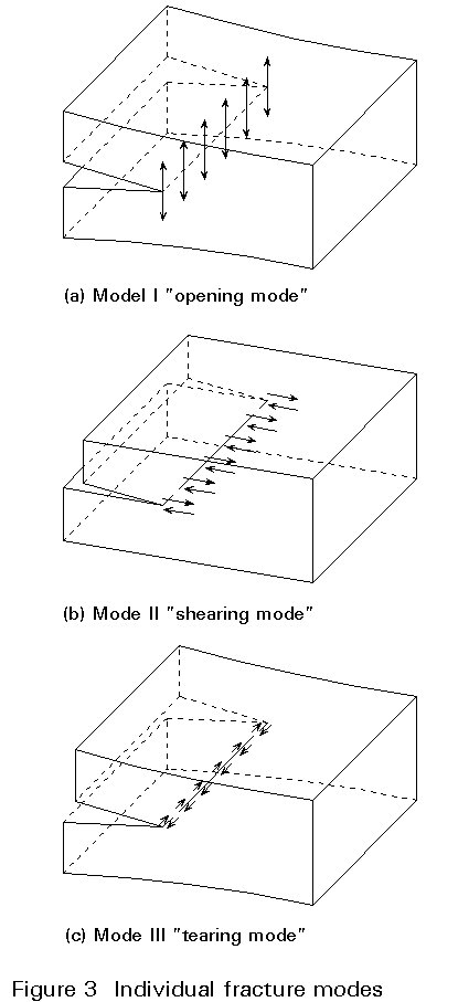
However, the predominant and most influential mode of cracking refers to mode I named the opening mode. This mode of cracking governs most of the fatigue crack behaviour encountered in practice for steel structures.
Applying the same methods developed earlier, similar expressions for the stress field derived for mode I, may be obtained for mode II and mode III. These expressions are given in a schematic format below; KII and KIII are respectively the stress intensity factors for mode II and mode III. These stress intensity factors depend only upon loading and geometric configuration. Relations for the displacement and the strain fields are not given, but they are easily obtained from the equations of the theory of elasticity in terms of the stresses.
Mode II
 (3.1)
(3.1)
for plane strain szz = u (sxx + syy) ; sxz = syz = 0
for plane stress szz = sxz = syz = 0
Mode III
 (3.2)
(3.2)
s
xx = syy = szz = sxy = 0The solutions which were derived, for determining the stress field at the crack tip, are based on linear-elastic theory. Equation (2.11) shows that, when r ® 0, the stress at the crack tip becomes infinite; this has no physical meaning. Therefore, at the front of the crack tip there will always be a localized plastic deformation which will affect the crack behaviour, i.e. the crack growth rate. The size of this plastic deformation at the front of the crack is discussed below.
At the crack front there is always a localized plastic deformation which will affect the growth of the crack. The first attempt which was made to predict the size of the plastic zone in the front of a crack was reported by Irwin. He proposed a very simple model. Referring to the same Griffith reference case, the elastic stress syy along the x axis at the front of the crack (Figure 4a) using plane stress theory is given by (see Equation (2.11)):
![]() (4.1)
(4.1)
where s is the stress in the y direction at infinity.
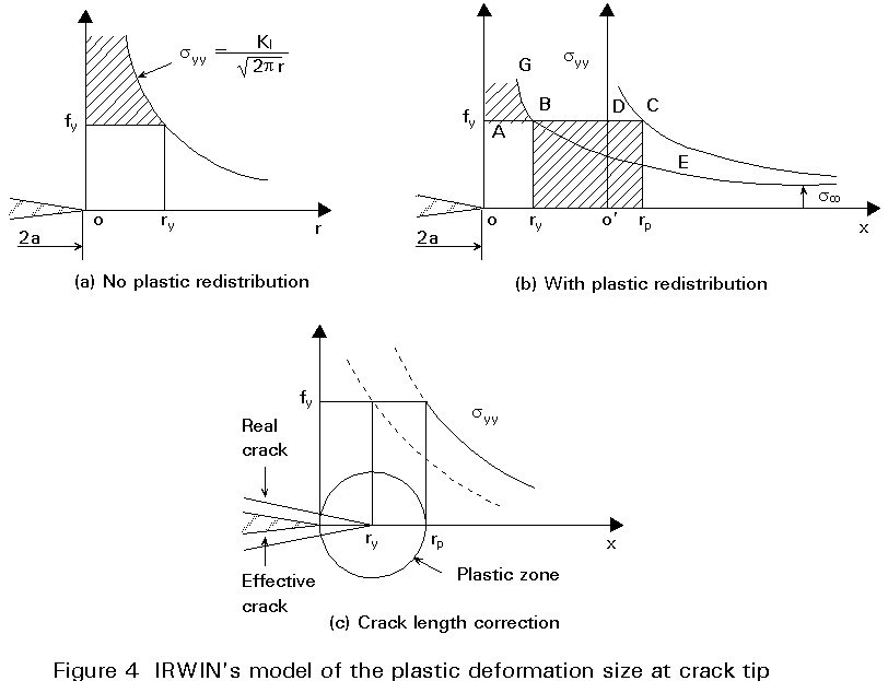
Let fy be the elastic limit of the steel plate material; the elastic stresses are, therefore, limited by:
![]() (4.2)
(4.2)
from which the size of the plastic zone can be predicted
ry = 1/2p (KI/fy)2 (4.3)
For plane strain theory, ry becomes:
ry = 1/2p [KI (1 - 2 u)/fy]2
However, this reasoning is very simple, and is not representative of reality. In setting up the inequality (Equation (4.2)) it was considered that no stress redistribution due to plastic deformation takes place within the plate. Consequently the plastic deformation size along the x axis cannot be the one represented on Figure 4a. The size of the plastic deformation zone, allowing for stress redistribution, must be greater. Suppose that the elastic stress curve has been shifted to the right by a quantity 00¢ (the stress curve being translated by the vector (00¢ ) (Figure 4b). The stress distribution syy along the x axis is expressed by:
syy = fy for x £ rp
and (4.4)
![]() for x > rp
for x > rp
In order to estimate the plastic deformation zone allowing for stresses redistribution, Irwin made the assumption that the total elastic area GBE, in other words the elastic energy, is equal to the elasto-plastic energy represented by the area ACF.
From consideration of the geometry the following equality may be written:
![]() (4.5)
(4.5)
Therefore
Hence
![]() (4.6)
(4.6)
Taking into account Equation (4.3), Equation (4.6) becomes:
![]()
Figure 4c gives a schematic representation of the plastic zone, and the associated effective crack length (a + ry), the size of the plastic zone being equal to 2 ry.
If the simple model of Irwin empirically takes into account the stress redistribution, it ignores completely the presence of the other stresses sxx and syy.
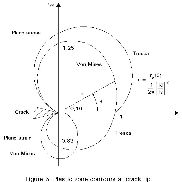
Designating s1, s2 and s3 the principal stresses, the von Mises criterion is
(s1-s2)2 + (s2-s3)2 + (s3-s1)2 = 2 fy2 (4.7)
in which
s
1 = 1/2 (sxx + syy) + 1/2s2 = 1/2 (sxx + syy) + 1/2 ![]() (4.8)
(4.8)
and s3 = 0 (plane stress)
s3 = u (s1 + s2) (plane stress)
Substituting Equation (2.11) for mode I in Equation (4.8) and in Equation (4.7) gives:
rp = (1/2p) (KI/fy)2 cos2 q/2 (1+3 sin2 q/2) (4.9)
rp = (1/2p) (KI/fy)2 [(1-2u)2 + 3 sin2 q/2] (4.10)
The Tresca criterion is based on the maximum shear tmax and is written as:
t
max = 1/2 fy (4.11)where
A similar derivation to that above leads to the following equations:
rp = (1/2p) (KI/fy)2 cos2 q/2 (1+ sin q/2)2 (4.13)
rp = (1/2p) (KI/fy)2 cos2 q/2 max [1, (1-2u +sin q/2)2] (4.14)
This yielding model ahead of a front crack due to D S Dugdale (1960) deserves to be presented since it introduces the crack opening displacement concept (COD). Consider again the Griffith problem, and suppose that the yielding spreads at both crack lips on a distance w (Figure 6a). This short yielded distance w may be easily determined, considering the following superposition of stress fields.
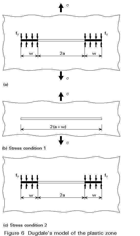
Support that the crack of length 2(a + w) is subjected to a tensile stress s applied at the infinity. This is referred in Figure 6 as stress condition 1. A second stress condition may be considered where two distributed compressive field stresses are opening both crack lips over the distance w, referred in Figure 6c as stress condition 2. Superposing the stress condition 2 with the stress condition shown in Figure 6a, gives stress condition 1. The stress intensity factor of a through-crack length 2(a + w) in an infinite body is:
![]() (5.1)
(5.1)
In the case of stress condition 2, the stress intensity factor may be easily obtained from the Green function of the solution relative to a pair of concentrated opening forces acting symmetrically on the two lips of a crack (cf. Lecture 12.12). Therefore, the solution is:
![]() (5.2)
(5.2)
The sum of the stress intensity factors KI1 and KI2 must be equal to zero. Then the plastic zone dimension w is:
w = -a + a / cos |sp/2fy| (5.3)
By developing cos |sp/2fy| in series when s << fy, and taking the first term of the series gives:
cos |sp/2fy| » {1 - |s/fy|2.p/8} (5.4)
The dimension of the plastic zone may be obtained from Equation (5.2) taking into account Equations (5.3) and (5.4), then
w = p/8 |K1/fy|2 w = p/8 {K1/fy}2 (5.5)
This value is very near to the solution obtained by Irwin (see Equation (4.3)). When the ratio (s /fy) becomes greater the difference between the two solutions increases.
Burdekin and Stone [6], according to the approach outlined in paragraph 2.1, calculated the displacement d at the end of the real crack (i.e. for x = ± a) and found:
 (5.6)
(5.6)
In the concept of the crack opening displacement approach, the crack propagates when d reaches its critical opening displacement dc which is a characteristic of the material.
From Equation (5.6) the critical stress corresponding to the Griffith problem is obtained knowing the critical opening displacement. Developing cos {sp/2fy} in series, and keeping the first term Equation, (5.6) reduces to
![]() (5.7)
(5.7)
The COD definition, being the crack opening displacement at the interface of the elastic and plastic zones, is convenient for calculation purpose. However, it is not very easy to measure experimentally the value of the crack opening displacement.
For a stress field in a problem of plane elasticity:-
KI » Ö(2p) lim Sz-0 Z''Öz
A proper Z function must be selected, which satisfies the boundary conditions.
KI 2 = sÖ(pa)
Therefore, the distribution of stresses in a cracked body is an invariant with respect to the loading and geometries of the crack and the body. However, the magnitude of these stresses depends upon these two parameters which are taken globally in the KI value called the stress intensity factor in mode I. KI depends on the external loading, the overall geometry of the crack body, and on the crack geometry (dimensions and shape).
This factor should not be confused with the geometric stress concentration factor Kt which is, for a particular notch, the ratio of the maximum stress to the nominal stress. Kt is, therefore, a purely conventional coefficient, giving an indication of the stress concentration at a notch for particular conditions of geometry and loading.
In reality there will always be localised plastic deformation at the front of the crack tip which affects crack behaviour:
The dimensions of the plastic zone ahead of a crack may be found using the yielding model of D S Dugdale:
[1] Eurocode 3: "Design of Steel Structures": ENV 1993-1-1: Part 1.1, General principles and rules for buildings, CEN, 1992.
[2] Timoshenko S, Goodier N.J., "Theory of Plasticity", McGraw Hill Book
Company, 2nd Edition, New York 1951
[3] Germain P, "Mcanique des Milieux Continus", Masson et Cie, Paris, 1962.
[4] Westergaard H.M., "Theory of Elasticity and Plasticity", Dover Publications, inc. New York, 1964
[5] Francois D., Joly L. (Ed.), La rupture des métaux, Masson et Cie, 1972
[6] Burdekin E.M., Stone D.E.W., The crack opening displacement approach to fracture mechanics in yielding materials Journal of Strain Analysis, vol. 1, no 2, 1966.