ESDEP WG 2
APPLIED METALLURGY
To describe the selection of steel quality in relation to requirements of toughness.
Lecture 2.1: Characteristics of Iron-Carbon Alloys
Lecture 2.3.1: Introduction to the Engineering Properties of Steels
Lecture 2.3.2: Advanced Engineering Properties of steels
Lecture 2.4: Steel Grades and Qualities
Lecture 2.6: Weldability of Structural Steels
Selection of the right steel quality for a structure is a matter of major significance as regards both the safety and the economy of constructional steelwork. This lecture surveys procedures which have been proposed for this purpose and presents the new rules which are included in Annex C of Eurocode 3 [1]. All these express, as a function of extreme service conditions applicable to a structure, a toughness level specified in terms of performance in the Charpy V test that the selected steel should fulfil, with a transition temperature at the level of 28J for instance. Numerous comparisons between the output of different procedures are reported which, on the one hand highlight their consistency, while on the other hand the possible sources of discrepancies among the various material requirements determined using these procedures. Such procedures are based on fracture mechanics concepts such as those of the Stress Intensity Factor, the Crack Tip Opening Displacement or the Full Yield Criterion. As an introduction the lecture reviews the main aspects of resistance to brittle failure, with reference to basic documents which the reader may find it useful to consult for more detail.
There are circumstances when the integrity of a structure is governed not by the strength of the metal but by another property, namely toughness.
Such situations generally imply the presence of defects in the structure such as cracks or sharp notches and are favoured by the occurrence of low temperature. The incidence of dynamic loads is another parameter enhancing the risk of so-called brittle fracture.
Thus the engineer has to consider that the concept of ultimate boundary states and the fulfilment of the related criteria may apply and lead to a safe design only if the pre-requisite conditions that prevent brittle failure are met.
In normal circumstances, it is impracticable to undertake a detailed 'fitness-for-purpose' analysis involving sophisticated fracture mechanics tests either at the design stage or during fabrication and erection of conventional structures. For such constructions, simple rules have to be developed and specified in building codes to define which qualities of steel should be selected to ensure a safe design.
This lecture is divided into sections devoted respectively to:
A material is generally said to be brittle if it cannot be deformed to any appreciable degree prior to fracture. This behaviour does not imply that the ultimate tensile strength measured on a smooth specimen during a tensile test is low. On the contrary, the opposite phenomenon is usually observed. Hardening treatments which aim to increase strength are usually accompanied by a dramatic degradation of ductility and tend to enhance brittleness.
Brittleness is neither an absolute nor a simple concept. As a rule, the susceptibility to brittle behaviour in a given material is increased by:
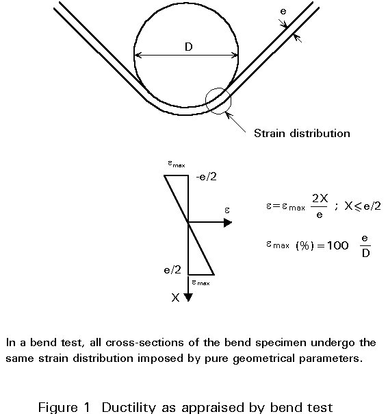
Brittleness is influenced by ductility, i.e. the capacity of a material to strain plastically, and by strain-hardenability, i.e. the property of developing a higher strength while undergoing plastic deformation.
Ductility can easily be appraised in a bend test under strain-controlled conditions where the material is bent round a mandrel with large plastic strains being induced in the outer fibres of the specimen (Figure 1). The more ductile material can be bent round a smaller mondrel without fracture.
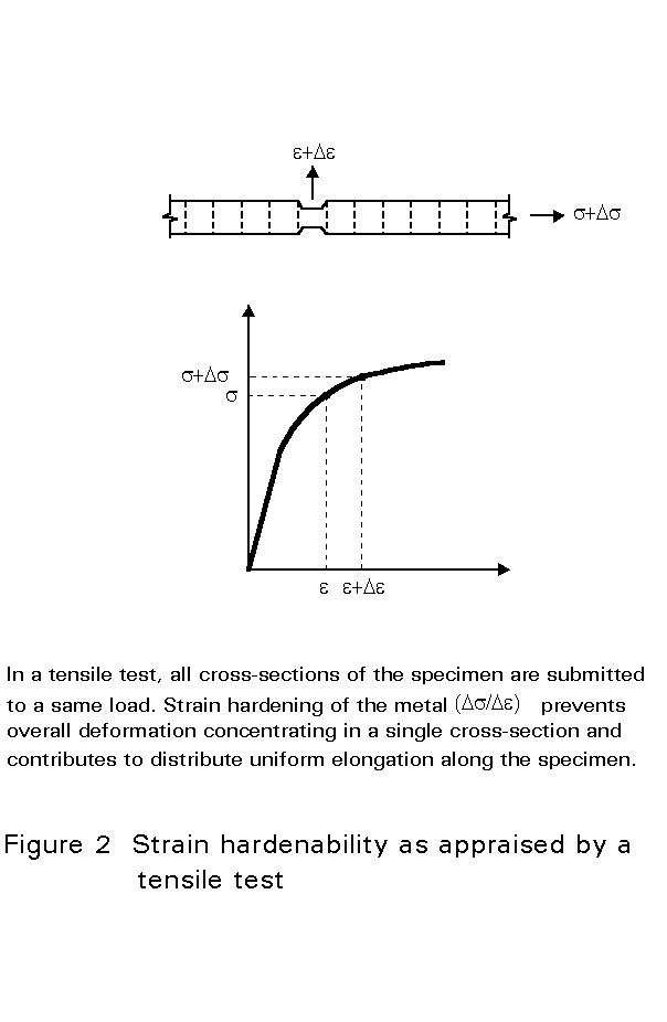
Strain-hardenability is appraised in a tensile test and is quantified by the slope of the stress-strain curve in the plastic regime. Strain hardening governs the amount of uniform elongation a material may undergo before necking or fracturing (Figure 2).
A material showing no ductility is intrinsically brittle and produces, even in a defect-free situation, negligible plastic elongation during a tensile test and no strain hardening. Such a material is glass.
Steel usually exhibits ductile behaviour in the tensile test and the presence of some defect is necessary to induce brittleness. The defect may be a geometrical discontinuity with sharp edges constituting a stress raiser, or an area in which the mechanical properties are locally impaired such as the heat affected zone of a weld, or a region of local plastic deformation which may undergo subsequent strain ageing. Often, both geometrical and metallurgical defects are present together; weldments may undergo lack of penetration or contain cold cracks, while punches or shears may create burrs or notches. A large embrittling effect may thus be induced.
Should the ductility of the metal at the tip of the notch be very poor, then no possibility would exist to blunt the notch by plastic deformation. The result would be a brittle failure occurring at a load which can be calculated from linear elastic theory as a function of the component dimensions, the notch size and the toughness characteristics of the metal.
In the case where a degree of ductility is available, crack blunting occurs and is reflected in a degree of crack opening. The fracture behaviour is then significantly influenced by the strain hardenability of the metal. If little strain hardening is available, then the crack may propagate through the component at a rather constant stress level, either by ductile tearing or brittle cracking.
Different fracture behaviour can be observed with a ductile metal which is capable of sustained strain hardening since propagation of the defect after crack blunting requires an increasing load to be applied to the component. Such conditions give rise to stable crack propagation.
Several specific tests have been developed to assess the fracture behaviour of materials in various loading conditions and defect configurations. It is not the scope of this lecture to detail the testing procedures or review the methods for derivation of toughness values. However, it is worth listing the main concepts and types of test as well as the assumptions on which they rely.
Fracture Mechanics has been approached in a rigorous way on the basis of linear elastic theory which led to the well-known concept of stress intensity factor, KI [2]. This parameter defines completely the stress field in the vicinity of a crack. Fracture occurs when it attains a critical value which is a characteristic of the material. The main assumption of this theory is the presence of minimal plastic strain at the crack tip. With steel, such conditions may be met with very high strength products or when the thickness is large. Table 1 defines the basic equations of Linear Elastic Fracture Mechanics (LEFM) together with the conditions of applicability.
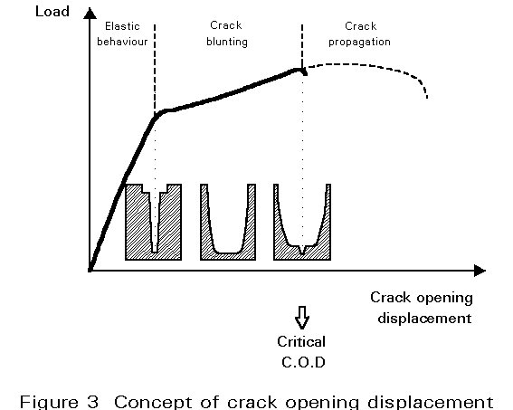
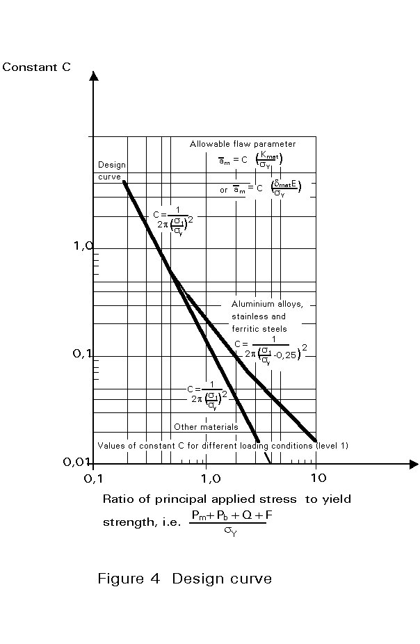
In many circumstances significant plasticity takes place at the crack front prior to failure and crack opening may be observed before fracture initiation (Figure 3). The concept of Crack Opening Displacement (COD) or more precisely (CTOD) defines the amplitude of the crack tip plasticity under a given stress situation. Fracture initiates when this parameter reaches a critical value (dcrit) which is a characteristic of the material and a measurement of its toughness [3].
The theory of the J integral is based on the same assumptions as above but computes a specific fracture energy whose value is independent of the contour of integration and which is an alternative measurement of the material toughness [4].
It is important to mention that both the CTOD and the J concepts are designed to assess situations in which fracture occurs in the elasto-plastic region, but imply nevertheless a relatively small extent of plastic strain at the crack tip. To assess the risk of failure by brittle fracture, means have been provided to estimate the CTOD or J values in a large structure containing a defect, as a function of the overall applied loads. These estimated values are then compared with the critical failure values for the relevant material. A well known design curve for such fitness-for-purpose analysis is based on the CTOD approach (Figure 4).
All the above procedures normally require that the product be tested with its full thickness so as to derive a suitable toughness index. Although this condition may involve test specimens having rather large dimensions, it can never be considered as appraising the overall fracture behaviour of a structural component. Therefore, the relevance of the transferability of the test data for the appraisal of large structures has to be verified by comparing the computed fracture behaviour to that experimentally observed during tests on a very large piece whose size is similar to the parts of a real structure.
The Wide Plate test has been designed with this aim. It involves tensile testing, possibly at lowered temperature, of a wide specimen (1m wide for instance) containing deliberate through-thickness or surface cracks. A convenient evaluation of performance in the Wide Plate test is provided by the Yield criterion [5]. When full yield occurs, then all sections of the specimen, even those not affected by the defect, develop plastic strains so that the overall elongation is sufficient to prevent a sudden failure. Full yield also ensures that the structure can reach its maximum elastic design load, i.e. the product of the material yield stress and the gross section, as if it were not affected by the defect, which is an obvious asset for safety. A critical defect length can be defined above which the criterion can no longer be fulfilled; then only net section yielding or contained yielding are achieved. Table 2 summarises the main concepts relating to the Wide Plate test.
There are situations in which resistance to failure is not governed by toughness but by the load bearing capability of the net section in the part affected by a defect. This situation may occur with quite ductile materials affected by cracks. Plastic collapse corresponds to the achievement of unlimited displacements in the net section when the applied load induces a net section stress equal to the material flow stress. A ratio Sr may be defined to express the safety against plastic collapse for a given loading condition. It is sometimes more convenient to use the material yield stress as a reference and think in terms of plastic yield load. A ratio Lr is then considered. Table 3 defines the parameters.
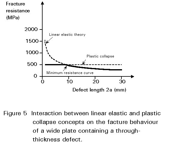
Although the assumptions associated with Linear Elastic Fracture Mechanics and Plastic Collapse lead to quite opposite fracture mechanisms, both concepts may actually apply to the same material and even the same structure depending on the defect size. Figure 5 illustrates this situation for the simple example of a wide plate containing a through-thickness defect. For small defect sizes the lowest fracture resistance is dictated by plastic collapse concepts, whereas for larger defects the lowest fracture resistance is obtained from linear elastic theory.
This interactive behaviour supports the so-called two-criteria approach developed by CEGB in 1976, and known as the R6 procedure, whose latest 3rd revision is now well developed [6]. A Failure Assessment Diagram (FAD) expresses the risk of failure in a two-dimensional space using the Sr or Lr parameter as the abscissa and a Kr variable as the ordinate. Kr is the ratio between the applied and critical KI stress intensity factors. Safe and unsafe conditions are discriminated by a curve quantifying the interaction. The main aspects of this method are summarised in Table 4.
Toughness properties of structural steels are generally classified in material standards such as the new EN 10025 [7] and EN 10113 [8] in terms of performance in the Charpy V test. While levels of absorbed energy may be defined for different test temperatures, a simple and classical characteristic often encountered is the Transition Temperature at the level of 28J: TK28
Any methodology for steel selection applicable to standardised steel grades must involve the following steps:
i. A definition of extreme service conditions against which to address the resistance to fracture of a structure, i.e. a size of defect, a mode of loading (static or dynamic) and a level of internal or external stress.
ii. A method of fracture analysis leading to the derivation of toughness requirements as a function of the above conditions.
iii. A relationship between the toughness requirements and a transition temperature or energy in the Charpy V test.
The different methods that are available are reviewed below.
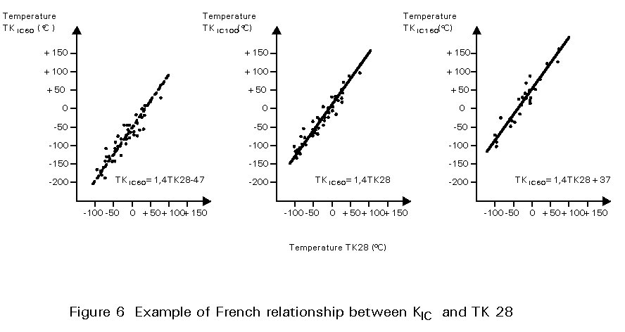
This procedure was designed by Sanz and co-workers at IRSID in the late seventies, elaborated by a Working Group of ATS and published in 1980 [9].
It is based on a set of experimental relationships between the transition temperatures in KIC and Charpy V tests, which are illustrated in Figure 6, which is reproduced from the original publication.
The analysis of the risk of brittle failure is based on Linear Elastic Fracture Mechanics, and toughness requirements are derived in agreement with this theory. Some modifications which were introduced for simplification purposes are highlighted in the document and result in more conservative assumptions.
A particular feature of the method lies in the fact that defect sizes are defined in relation to plate thickness so as to match with the conditions of plane strain and thus ensure the applicability of a LEFM approach.
The main steps involved in the definition and application of the SANZ method are summarised in Table 5. The final formula leading to the definition of steel quality in terms of a TK28 index takes account of the service temperature and the strain rate to which the structure may be exposed, as well as the scatter in the experimental relations.
Some predictions of the necessary transition temperature at the Charpy V level of 28J are illustrated in Table 6 for the condition of a structure operating at a minimum service temperature of 0°C and possibly loaded up to the material yield stress at a slow strain rate (έ = 0,1s-1).
This method conceived by George in the United Kingdom was first proposed to the International Institute of Welding in 1979 [10].
It relies on an elasto-plastic analysis of the fracture resistance using the CTOD design curve for a structure containing a surface flaw of 0,2 times the plate thickness, in a field having a high level of residual stress and loaded to 0,67 times the yield stress. The steel quality is defined in terms of the required Charpy V energy at the service temperature assuming a relationship between this energy and the critical CTOD value. The formula derived in this way was calibrated against results from wide plate tests and practical experience.
Table 7 reviews the main assumptions supporting the method and the mathematical relationships which are derived.
Toughness requirements for a range of steel grades and thicknesses are listed in Table 8.
Developed in the late 1980's, this method directly links the fracture behaviour of wide plates containing through-thickness defects which are tensile tested at temperatures between -10 and -50°C, to the following metal characteristics: tensile strength or tensile-to-yield ratio and Charpy V energy at the same temperature [11].
Net fracture stress of the wide plate is first expressed as a function of defect size in terms of a linear decreasing function whose ordinate at the origin precisely equals the tensile strength of the metal and whose slope is inversely proportional to the toughness expressed by the Charpy V energy. Figure 7 illustrates these relationships. Net fracture stress is then converted into gross section stress using the specimen width as a correction parameter. At that stage the critical defect size according to the full yield criterion is computed as the smaller positive root of a second order equation.
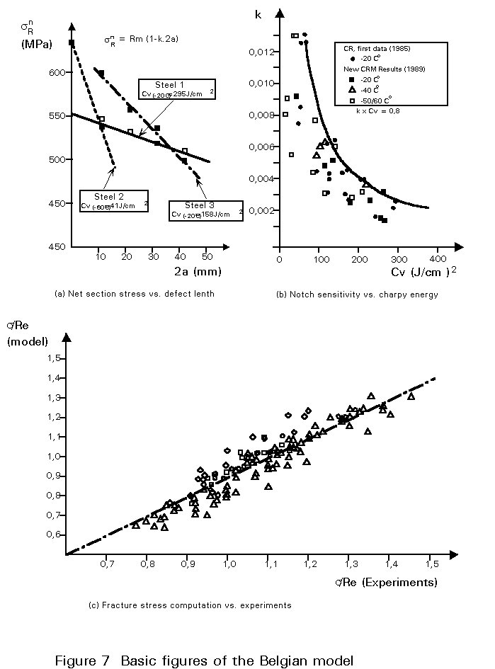
Table 9 lists the principal rules of the model which was originally developed to document the fracture behaviour of parent metal and later extended to appraise butt welded wide plates. In the latter case, local values of tensile strength and toughness of the metal at the crack tip are considered by using Charpy specimens with the notch root positioned in either the weld metal or the heat affected zone. Hardness measurements are carried out and converted into a proper Rm when this parameter cannot be directly derived from a tensile test. For plain or welded plates, the yield stress used in the formulae is always that of the base metal away from the crack.
The method for steel selection adopted in Eurocode 3 [1] results from a combination and a synthesis between the concepts proposed in the French method and the recommendations of CEGB [6]. The Eurocode procedure is described in recent publications [12, 13] and can be summarised as follows:
This approach considers three alternative stressing conditions (S1, S2, S3), two possible levels of strain rate (R1, R2) and two consequences of failure (C1, C2) which respectively allow distinction between:
(a) Lower or higher stresses, monolithic elements or welded joints, stress-relieved or as-welded structures, weaker or stronger effects induced by stress raisers.
(b) Quasi-static or rapid stressing conditions corresponding, on the one hand to permanent loads, actions of wind, waves or traffic, and on the other hand to impacts, explosions, collisions.
(c) Either ruptures leading only to localised damage not affecting human life and the stability of the whole structure, or failure whose local occurrence implies disastrous consequences for the global resistance of the structure or impairs the safety of people.
The Failure Assessment Diagram according to the R6 Rev. 3 [6] method which is taken into consideration is that corresponding to the so-called Option 2 which takes account of the actual tensile stress-strain curve of the steel. Figure 8 illustrates this diagram which in Eurocode 3 terminates at an abscissa having a value of unity [1].
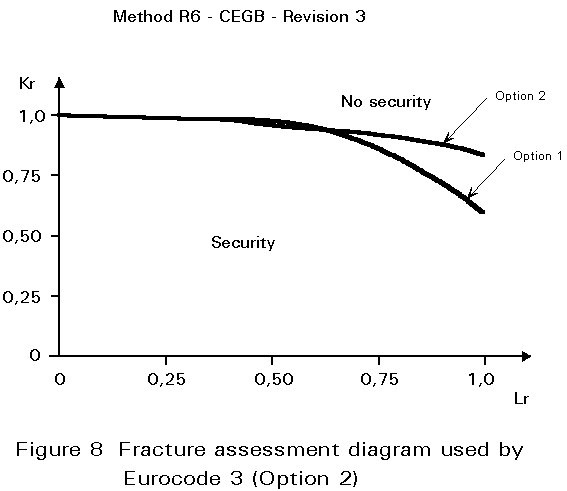
It is then supposed that the structure may contain semi-elliptical surface flaws whose size is proportional to the natural logarithm of the thickness (depth=ln t, length = 5ln t).
Critical Kr values are derived from the failure assessment diagram after computation of the relevant Lr for the different stress conditions. The necessary toughness, KIC that the material should display at the relevant service temperature can thus be readily defined.
The conversion of this requirement into a Charpy V TK28 transition temperature is finally carried out according to the French procedure.
Table 10 summarises the major aspects of the successive derivations. It highlights the fact that the strict application of this procedure for a given situation would first require a detailed fracture analysis according to the two-criteria approach so as to derive the necessary level of toughness required from the material in terms of a critical stress intensity factor here denoted Kmat. Such an analysis, which must include the respective contributions of the mechanical and residual stresses, as well as the correction factor for crack tip plasticity generated by the residual stress, should be carried out carefully according to a well-documented procedure such as that prescribed in British Standard PD6493 [14]. The critical stress intensity factor at the minimum design service temperature then has to be converted to a 28J transition temperature of a Charpy specimen. Here the rules defined by the French method are followed [9] so as to account for thickness and strain rate effects and the scatter in the relationship linking TKIC and TK28.
The procedure presented above should only be applied by specialists in fracture mechanics. On the other hand, the rules included in Eurocode 3 need to be applied by design engineers who require a more convenient formulation. With this aim in mind, the authors of the present Eurocode 3 rules have analysed a limited number of cases simulating the various loading conditions for different plate thicknesses, so as to derive, after a statistical analysis, a simplified formulation of the rules. The parameters of thee rules for practical application are listed in Table 11.
As an illustration of the rules, Tables 12 and 13 list a set of requirements for different values of yield stress and thickness corresponding to the S1, S2 and S3 load conditions as well as the C1 and C2 failure consequences.
Establishing a common basis for steel selection applicable internationally as a substitute for the existing national rules is a difficult task. Unifying a set of divergent specifications leads to new rules that are inevitably either less or more constraining than those defined in one or other of the national codes. On the one hand, concern may be raised against the reliability of the new rules with regard to a safe design, while on the other hand, criticism will be expressed towards an excessive degree of conservatism liable to spoil the economic competitiveness of constructional steelwork.
The present rules in Eurocode 3 [1] have informative status. To encourage as much as possible the concept of unified rules for steel selection, cooperation has been set up between the CEN/TC 250/SC3 Committee of Eurocode 3 and the International Institute of Welding who will study the problem on a multidisciplinary basis coordinated by Commission X with the support of Commission IX. An introductory article prepared by Professor Burdekin, Chairman of Commission X, was presented at the IIW 1992 annual assembly in this regard [15].
To contribute to the debate covering this important question, comparisons between the toughness requirements derived from the different approaches mentioned in this paper have been carried out and are presented below.
Available methods for steel selection differ in several respects: one of the most apparent is the form of the Charpy requirement which can be expressed either as a transition temperature or as a level of energy. Suitable conversion formulae are needed so as to perform comparisons between such methods.
Another factor of divergence is the definition of the flaw size as a function of plate thickness. Account must be taken of these differences when attempting to compare the various requirements.
Nevertheless, the main difference between the different approaches may arise from the assumptions which are made concerning the definition of the fracture model. The French approach is based on a purely linear elastic analysis, while the British and Belgian ones assume respectively elasto-plastic and full plastic behaviour of the structure. Another source of discrepancy could arise from the fact that the available methods were set up at different times and thus were calibrated on populations of steels which could differ widely in terms of chemical composition and processing route.
A major result that should emerge from the comparative exercises is therefore verification of whether the different concepts governing the existing approaches are able to generate consistent conclusions or, on the contrary, lead to contradictory outputs. It is clear that, if the latter situation should apply, little confidence could be shown in those models. Their significance would be restricted to the limited set of conditions and the generation of steels which were used during their formulation.
If consistent specifications can be derived from several models, another dimension would be conferred to the problem since, not only the overall reliability of the specifications would be enhanced, but sources of minor deviations could be better documented.
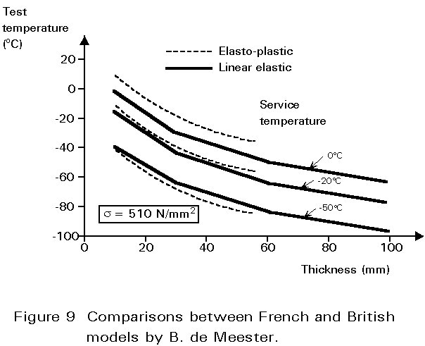
A significant step in highlighting the possible coherence of Charpy V based specifications was achieved by de Meester who presented valuable comparisons between the French and British approaches in 1986 [16]. An illustration of that work is reproduced in Figure 9.
A similar approach can be used to expand this evaluation to other methodologies. It will be recalled that some procedures express the necessary toughness in terms of a transition temperature while others require a level of energy at the service temperature. Means of conversion are, therefore, necessary in such cases. Table 14 reproduces the equations which were adopted in [16] on the basis of extensive comparisons reported in the 1970's [17].
Further information is necessary in order to make comparisons with the Belgian method since this procedure requires, as an entry parameter, the tensile-to-yield stress ratio of the relevant steel. This parameter depends, among other things, upon the processing route undergone by the material. A characteristic value cannot therefore be defined for a given steel grade. Typical values may, however, be considered on a statistical basis as a function of the guaranteed yield stress, such as those illustrated in Figure 10 which were proposed by Dahl and his co-workers [18]. Such a relationship is used in the present analysis to establish the necessary comparisons. Taking into account that thicker plates generally display a higher Rm/Re ratio than thinner products, data corresponding to the lower boundary or those closer to the upper side of the relationship of Figure 10 are selected depending on the thickness.
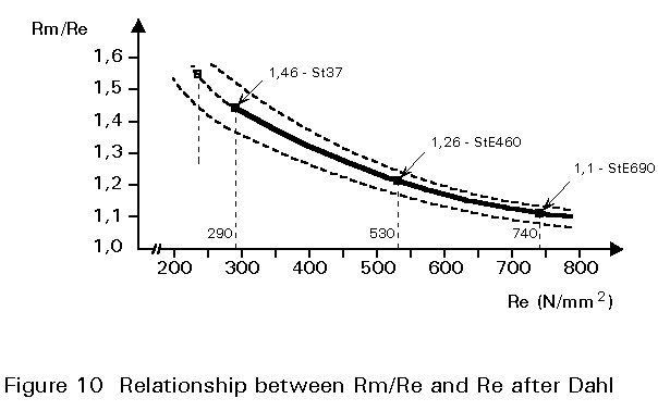
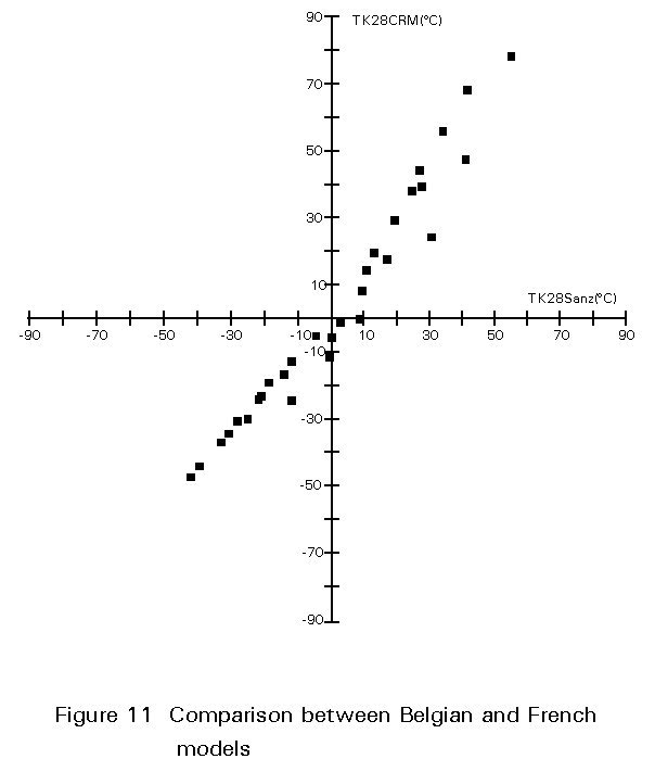
Table 15 lists the toughness requirements obtained from the Belgian method applied with same defect sizes as those considered in the French procedure (cf Table 6). TK28 transition temperatures required by both models are compared in Figure 11, which highlights the coherence of the respective specifications, especially in the significant field of negative transition temperatures, which represent the most severe conditions to be fulfilled by the material.
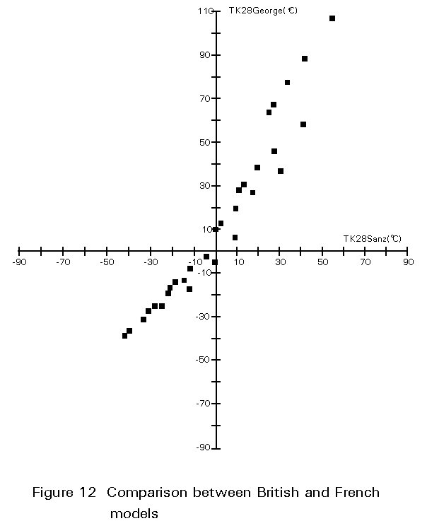
A comparison between the French and British methods is provided in Figure 12 using data which were generated in Tables 6 and 8. Here again specifications from both models are consistent. It will, however, be noticed that the French procedure considers smaller defect sizes (as a function of thickness) than the British method, for instance 8mm against 12mm for a 30mm thick member. This means that, for the same flaw size, the elasto-plastic fracture analysis developed by George on the basis of the design curve and Charpy COD relationships would lead to steel toughness requirements that were somewhat less stringent than those defined by the linear elastic approach of Sanz and the TKIC-TK28 relationships.
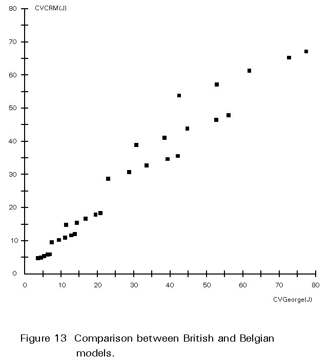
A similar conclusion is reached when roughly comparing, on a same defect size basis, the British rules to the Belgian procedure. Considering, however, that the George model assumes a design stress of only 2/3 of the yield stress and implementing this stress level in the CRM model, quite consistent requirements between both methods would be obtained. This is highlighted in Figure 13 which is drawn with data extracted from Tables 8 and 16.
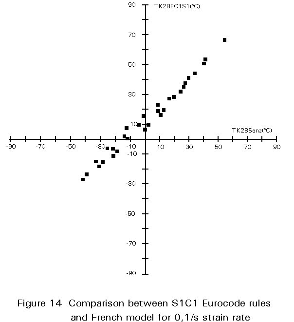
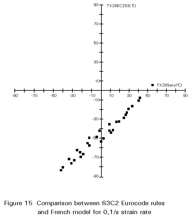
Requirements derived from the present Eurocode rules are compared to those from the French rules using the data listed in Tables 6 with Table 17 (S1 loading and failure condition C1) and Table 18 (S3 loading and failure condition C2). It is important to note that for the sake of consistency regarding the effect of strain rate, the same value of 0,1s-1 has been adopted for all procedures. Figures 14 and 15 illustrate that, depending on the loading conditions and failure consequences, Eurocode 3 rules are either less stringent or, on the contrary, significantly more constraining than the specifications of the French standard from which they are partly derived.
The comparison exercises reported above have demonstrated that, although the models were derived from quite different basic assumptions and fracture concepts, and were validated at different periods on different steel qualities and steel generations, the French, British and Belgian models lead to consistent Charpy requirements. This agreement is reached when the procedures are compared to each other on a carefully balanced basis, i.e. adopting the same defect size as a function of plate thickness and the same stress level. The strain rate is an important factor, which is an explicit parameter in the French method but not in either of the others. The Belgian model does, however, take some account of this effect through the tensile-to-yield ratio which is influenced by the strain rate sensitivity of the material. All comparisons with the French model were carried out for the slow strain rate of 0,1s-1 with a view to improving consistency. It is nevertheless clear that the strain rate sensitivity may vary, not only as a function of the steel grade, but also according to the applied processing route or chemical composition. This parameter would certainly be worth being better documented so as to optimise the rules for steel selection in certain applications involving dynamic effects.
The major sources for possible divergence between the existing rules have been identified. Many specifications are based on their conventions regarding the evolution of the admissible defect as a function of member thickness and the prevailing state and level of stress. This results in the definition of less or more stringent requirements. Such a situation becomes disturbing and confusing when the procedure that the fabricator has to follow is not properly documented in those terms, or when the computational steps are complicated and do not easily provide the possibility of carrying out even a limited parametric analysis.
Simple rules involving clearly defined models and based on rigorous mathematical treatments, ideally developed into analytical formulae, should constitute a preferred choice in the establishment of steel selection criteria. On the other hand, complex methodologies involving advanced concepts of fracture analysis may be misleading since their practical application would either be too difficult or simplification of the procedure would result in the infringement of basic fracture mechanics rules.
Eurocode 3 rules have been reviewed as well as the philosophy that prevailed in their development. Comparisons with the French model on which they are partly based, reveal overall agreement in a large range of transition temperatures, together with the possibility of shifting widely the requirements depending on the stress conditions (3 levels), the strain rate (2 conditions), and the consequences of failure (2 conditions): Tables 12 and 13 show that between S1R1C1 and S3R2C2 conditions, the difference in required TK28 temperatures is equal to or greater than 90°C.
These rules still require improvement and need to be discussed within a large forum of specialists. The cooperation of the International Institute of Welding in this task will bring a worldwide dimension to the challenge of unifying the rules for steel selection. Initial proposals for a coordinated approach to the problem were formulated at the IIW annual assembly of 1992 [15].
It may be of interest in this regard to quantify roughly how each of the available models accounts for variations of the plate thickness or of the steel yield stress on the TK28 requirements, all other factors being unchanged. In practice a significant question is to evaluate the advantages of implementing in a given type of structure, higher strength steels with thinner gauge as an alternative to conventional grades in thick sections. With this aim, the TK28 requirements listed in the various Tables 6, 8, 12, 13 and 15 have been correlated by linear regression analysis to thickness and yield stress so as to derive the following expression for each model:
TK28 = a - b.e - c.Re
The following b and c coefficients were derived:
|
French model |
b = -0,64 |
c = -0,12 |
|
British model |
b = -0,99 |
c = -0,12 |
|
Belgian model |
b = -0,85 |
c = -0,12 |
|
Eurocode model |
b = -0,54 |
c = -0,15 |
These values indicate that the French, British and Belgian rules seem more favourable for the adoption of higher strength steels and thinner gauges than the Eurocode specifications.
[1] Eurocode 3: "Design of Steel Structures": ENV 1993-1-1: Part 1.1, General rules and rules for buildings, CEN, 1992.
[2] Brock, D., Elementary engineering fracture mechanics, Martinus Nijhorff Publishers, 1987.
[3] Garwood, S. J., A crack tip opening displacement (CTOD) method for the analysis of ductile materials, ASTM STP 945, June 1985.
[4] Rice, J. R., A path independent integral and the approximate analysis of strain concentrations by notches and cracks, Trans. ASME, J. Appl. Mech. 1968, 35 379-386.
[5] Soete, W. and Denys, R., Evaluation of butt welds based on a strain criterion, Revue de la Sodure, Lastijd schrift, No. 4, 1975.
[6] Milne, I., Ainsworth, R. A., Dowling, A. R., Stewart, A. T., Assessment of the integrity of structures containing defects, CEGB document R/H/R6 - Revision 3, May 1986.
[7] EN 10025: Hot Rolled Products of Non-alloy Structural Steels and their Technical Delivery Conditions, British Standards Institution, 1990.
[8] EN 10113-1: Hot Rolled Products of Weldable Fine Grain Structural Steels Part 1: General Delivery Conditions, British Standards Institution, 1993.
ENV 10113-2: Hot Rolled Products of Weldable Fine Grain Structural Steels Part 2: Delivery Conditions for Normalized/Normalized Rolled Steels, British Standards Institution, 1993.
ENV 10113-3: Hot Rolled Products of Weldable Fine Grain Structural Steels Part 2: Delivery Conditions for Normalized/Normalized Rolled Steels, British Standards Institution, 1993.
[9] Sanz, G., Essai de mise au point d'une mthode quantitative de choix des aciers vis-á-vis du risque de rupture fragile, Revue de Mtallurgie - CIT, Juillet 1980.
[10] George, M., A method for steel selection, Document IIW-IXF.
[11] Defourny, J., D'Haeyer, R., Leroy, V., A metallurgical approach of the parameters affecting the fracture behaviour of base metal and welded components, IIW document IX-1607-90/X-1206-90.
[12] Sedlacek, G., Bild, J., Hensen, W., Background document for Chapter 3 of Eurocode 3 "Design Against Brittle Fracture", Aachen 1990.
[13] Brozzetti, J., Sedlacek, G., Hensen, W., Fondements des regles de l'Eurocode 3 en vue de se garantir du risque de rupture fragile, Construction Mtallique, no. 1, 1991.
[14] Guidance on methods for assessing the acceptability of flaws in fusion welded structures, PD6493: 1991, BSI.
[15] Burdekin, F. M., Materials selection for welded structural steelwork in Engineering Design in welded constructions, Pergamon Press, 1992.
[16] de Meester, B., The brittle fracture safe design of welded constructions, Welding in the world.
[17] Sanz, G., La rupture des aciers, fascicule 2, Collection IRSID OTUA.
[18] Dahl, W., Hesse, W., Krabiell, A., Zur WVerfestigung von Stahl und dessen Einflub auf die Kennwerte des Zugversuchs; Stahl und Eisen 103 (1983), Heft 2, Seite 87-90.
Table 1 Linear Elastic Fracture Mechanics
The three modes of loading at a crack tip:
The stress field around the crack is defined by a parameter K:
su = [KI /Ö(2pt)].fu(q) in mode I
Infinite plate: KI = sÖ(pa)
Finite plate of width W:
KI = sÖ(p a).[sec p a/W]
Through thickness crack in Mode I
Semi-elliptical crack:
KI = 1,12sÖ{pa/[f2 - 0,212(s/Re)2]}
f = Ö{1 - [(c2-a2)/c2].sin2j dj - 3p/8 + pa2f/8c2
Table 2 Concepts Associated with the Wide Plate Test

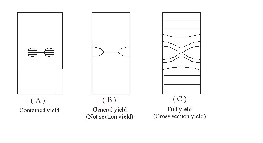
Gross section stress: sb = F/(W ´ t)
Net section stress: sn = F/[(W - 2a) ´ t]
sb = sn[1 - 2a/W]
Full yield : sb = Re
General yield : sn = Re
Determination of the critical defect length at full yield. Different wide plate tests are carried out at the same temperature but with different crack sizes.
Table 3 Plastic Collapse Concept
According to the plastic collapse concept, the load bearing resistance of the structure affected by a defect equals the product of the material flow stress by the net section.
The diagram below plots the gross stress at plastic collapse in a plate containing a through-thickness defect as a function of the 2a/W ratio (defect length to plate width).
Re : material yield stress
Rf : material flow stress
Rm : material tensile strength
Re < Rf £ Rm
Rf ~ (Rm + Re) / 2
s
b : gross stress applied to the wide plateSr = applied load/plastic collapse load = (sb / Rf) (1-2a/W)
Lr = applied load/plastic yield load = (sb / Re) (1-2a/W)
At plastic collapse
Sr = Srmax = 1 Lr = Lrmax = Rf/Re
Table 4 Main Rules of the R6 Procedure
|
Box 1: The R6 Rev. 3 Failure Assessment Diagram |
|
|
The simplifying concepts behind the R6 procedure are the two criteria for failure, characterised by: 1. Crack tip failure, where failure occurs when the applied load equals the LEFM failure load,
2. Failure by plastic collapse, defined when the load equals the plastic collapse load and the displacements in the structure become unlimited. The plastic collapse load may be formally defined as the load when the reference stress reaches the material's flow stress, . The criterion for plastic collapse failure is given by the ratio Sr. where Sr =
and this criterion was used for the initial R6 FAD. It is often more convenient to think in terms of plastic yield loads rather than collapse loads as it is easier to define and calculate these theoretically. In R6 Rev. 3 the ratio Lr is used as Lr = From this, the load for plastic collapse is given as Lrmax. With The simplest FAD requires that Kr < 1 and Lr < Lrmaz. |
This ignores any interaction between the two failure mechanisms. This interaction may be allowed for by writing the first inequality as Kr < f(Lr) and choosing an appropriate function for f. One such function is f(Lf) = where Je is the elastic component of J given by K2/E. Thus when sref is low, J = Je and f(Lr) = 1, consistent with LEFM failure. When s ref is high, on the other hand, failure is governed by J. Equation 5 may be used to generate an FAD directly from the load displacement curves of specimen tests. The most general method for calculating equation 5 is to use the reference stress procedures so that f(Lr) may be calculated directly from the material's stress strain curve. The general equation for this is f(Lf) = where eref is taken from the material's true stress - true strain curve at respective values of sref. The figure 6 is a plot of equation 6 as a function of Lr, using an experimental stress strain curve for a stainless steel. Although equation 6 is the preferred option for R6 Rev. 3, it requires a detailed knowledge of the stress strain curve of the material, especially around the material's yield point. In some cases, especially when dealing with hold plant, such knowledge is not available. Other options of the FAD have been developed for use in such circumstances. |
|
|
|
Table 5-1 Main Rules of the French Model
Between KIC and Charpy V based on Transition Temperature at respectively 100MPa Öm and 28 J:
![]() (S1)
(S1)
Plane strain condition,
![]() (S2)
(S2)
where e is in metres
Material yield stress Re, then
![]() (S3)
(S3)
where a is in metres
and from Equation (S2)
![]() (S4)
(S4)
For thick plates, a semi-elliptic surface defect 50mm long, 25mm deep, which is equivalent to a 28mm long through thickness defect (a = 14mm).
477 MPa is the yield stress level derived from S3 with a = 14mm and KIC = 100 MPa Öm.
110mm is the thickness satisfying Equation (S4) with a = 14mm.
Table 5-2 Main Rules of the French Model
For thick products (e ³ 110mm), a 28mm long defect corresponds to 100 MPa Öm at a yield stress of 477 MPa. For other values of Re, the following KIC values apply, as derived from Equation (S3):
|
Re (MPa) |
280 |
350 |
410 |
470 |
510 |
640 |
740 |
|
KIC (MPa Öm) |
59 |
73 |
86 |
99 |
107 |
134 |
155 |
To satisfy Equation (S4) the defect length is related to plate thickness as indicated by the following table. This table also lists the corresponding KIC values at a reference yield stress of 477 MPa.
|
e (mm) |
10 |
20 |
30 |
60 |
80 |
110 |
>110 |
|
2a (mm) |
2,5 |
5 |
7,5 |
15 |
20 |
28 |
28 |
|
KIC (MPa Öm) Re = 477 MPa |
30 |
43 |
52 |
74 |
85 |
100 |
100 |
Taking account of the above tables, it is necessary to consider transition temperatures for KIC values other than 100, but ranging between 30 and 160MPaÖm. This can be quantified through the following equation:
![]() (S5)
(S5)
Table 5-3 Main Rules of the French Model
Equation (S1) is used to relate a minimum service temperature above which the structure is safe to a required toughness level expressed as a transition temperature of 28J in the Charpy test.
The minimum service temperature is equal to TKIC = 100 for a structure made of a steel with reference yield stress 477 MPa, reference thickness 110mm and affected by the reference defect length a = 14mm.
For other values of yield stress or thickness, other values of KIC apply and corrections are introduced through Equation (S5).
Corrections are also made to take account of strain rate effects and the scatter in Equation (S1).
The final relationship is expressed as follows:
![]() (S6)
(S6)
in which
TS : minimum service temperature for fracture safe design
TK28 : transition temperature of Charpy V at 28J
b
(Re) : 60 lnD
Te : in theory, 60 1nD
TV : (83 - 0,08 Re) e 0,17 where is the strain rate in s-125 : scatter of Equation (S1)
Table 5-4 Main Rules of the French Model
The necessary steel quality expressed in terms of the 28J transition temperature is derived as a function of service temperature, strain rate, stress applied to the structure, material yield stress and thickness from the following formula:
Table 6 Some Results of the French Method
|
Re |
e |
2a |
b |
Te |
Tv |
TK28 @Ts=0°C |
|
(MPa) |
(mm) |
(mm) |
(°C) |
(°C) |
(°C)@0,1/s |
(°C) |
|
280 |
10 |
3 |
-49 |
-92 |
41 |
53 |
|
280 |
20 |
5 |
-49 |
-73 |
41 |
39 |
|
280 |
30 |
8 |
-49 |
-58 |
41 |
29 |
|
280 |
60 |
15 |
-49 |
-29 |
41 |
8 |
|
280 |
80 |
20 |
-49 |
-16 |
41 |
-1 |
|
280 |
110 |
28 |
-49 |
0 |
41 |
-12 |
|
350 |
10 |
3 |
-27 |
-92 |
37 |
40 |
|
350 |
20 |
5 |
-27 |
-73 |
37 |
27 |
|
350 |
30 |
8 |
-27 |
-58 |
37 |
16 |
|
350 |
60 |
15 |
-27 |
-29 |
37 |
-4 |
|
350 |
80 |
20 |
-27 |
-16 |
37 |
-14 |
|
350 |
110 |
28 |
-27 |
0 |
37 |
-25 |
|
410 |
10 |
3 |
-13 |
-92 |
34 |
33 |
|
410 |
20 |
5 |
-13 |
-73 |
34 |
19 |
|
410 |
30 |
8 |
-13 |
-58 |
34 |
9 |
|
410 |
60 |
15 |
-13 |
-29 |
34 |
-12 |
|
410 |
80 |
20 |
-13 |
-16 |
34 |
-22 |
|
410 |
110 |
28 |
-13 |
0 |
34 |
-33 |
|
480 |
10 |
3 |
0 |
-92 |
30 |
26 |
|
480 |
20 |
5 |
0 |
-73 |
30 |
12 |
|
480 |
30 |
8 |
0 |
-58 |
30 |
2 |
|
480 |
60 |
15 |
0 |
-29 |
30 |
-19 |
|
480 |
80 |
20 |
0 |
-16 |
30 |
-28 |
|
480 |
110 |
28 |
0 |
0 |
30 |
-39 |
|
510 |
10 |
3 |
5 |
-92 |
29 |
24 |
|
510 |
20 |
5 |
5 |
-73 |
29 |
10 |
|
510 |
30 |
8 |
5 |
-58 |
29 |
0 |
|
510 |
60 |
15 |
5 |
-29 |
29 |
-21 |
|
510 |
80 |
20 |
5 |
-16 |
29 |
-30 |
|
510 |
110 |
28 |
5 |
0 |
29 |
-42 |
|
Conditions: loading up to yield stress at a slow strain rate (0,1/s) |
||||||
Table 7 Main Rules of the British Model
Between the critical crack opening displacement (d in mm) of a material at a given temperature and the Charpy V energy (CV in Joules) at the same temperature:
![]() (G1)
(G1)
Fracture behaviour analysis according to the assumptions that prevail for the definition of the "Design Curve" in British Standard PD 6493, which for stainless and ferritic steel is expressed as follows:
 (G2)
(G2)
In the original model, a value of s equal to 1,9 Re was adopted as the result of the superimposition of a design stress equal to 0,67 Re affected by a stress concentration factor of 1,2 and a residual stress of amplitude equal to Re.
![]() (G3)
(G3)
A surface crack size 0,2 times the plate thickness deep and 1 times the thickness long, which corresponds to an equivalent crack size of 0,2e
![]() (G4)
(G4)
Combining Equations (G1) to (G4) leads to:
![]() (G5)
(G5)
equivalent to:
![]() (G6)
(G6)
Table 8 Some Results of the British Method
|
Re |
e |
2a |
CV |
TK28@Ts=0°C |
|
(MPa) |
(mm) |
(mm) |
(J) |
(°C) # |
|
280 |
10 |
4 |
4 |
106 |
|
280 |
20 |
8 |
8 |
58 |
|
280 |
30 |
12 |
12 |
37 |
|
280 |
60 |
24 |
24 |
6 |
|
280 |
80 |
32 |
32 |
-5 |
|
280 |
110 |
44 |
43 |
-17 |
|
350 |
10 |
4 |
5 |
88 |
|
350 |
20 |
8 |
10 |
46 |
|
350 |
30 |
12 |
15 |
27 |
|
350 |
60 |
24 |
30 |
-3 |
|
350 |
80 |
32 |
39 |
-14 |
|
350 |
110 |
44 |
54 |
-26 |
|
410 |
10 |
4 |
6 |
77 |
|
410 |
20 |
8 |
12 |
38 |
|
410 |
30 |
12 |
17 |
20 |
|
410 |
60 |
24 |
35 |
-9 |
|
410 |
80 |
32 |
46 |
-20 |
|
410 |
110 |
44 |
64 |
-31 |
|
480 |
10 |
4 |
7 |
67 |
|
480 |
20 |
8 |
14 |
31 |
|
480 |
30 |
12 |
20 |
13 |
|
480 |
60 |
24 |
41 |
-15 |
|
480 |
80 |
32 |
54 |
-26 |
|
480 |
110 |
44 |
74 |
-37 |
|
510 |
10 |
4 |
7 |
64 |
|
510 |
20 |
8 |
14 |
28 |
|
510 |
30 |
12 |
22 |
10 |
|
510 |
60 |
24 |
43 |
-17 |
|
510 |
80 |
32 |
57 |
-28 |
|
510 |
110 |
44 |
79 |
-39 |
|
#TK28 was derived from CV using formula (ET5) of Table 14 |
||||
Table 9 Main Rules of the Belgian Model
Between net fracture stress in wide plate test containing a through-thickness defect and Charpy V energy at the same temperature:
![]() (C1)
(C1)
where CV is expressed in J and not in J/cm² as in the original model.
Fracture appearance transition temperature in the Charpy test is lower than the temperature of the wide plate test.
Material yield stress on gross-section (the model may nevertheless be applied to other stresses).
![]() (C2)
(C2)
Length of the through-thickness defect (critical size) satisfying the full yield behaviour, expressed by the following equation:
![]() (C3)
(C3)
 (C4)
(C4)
Table 10-1 Main Aspects of the Eurocode Rules
Step 1.1 Definition of Stress Levels S1, S2, S3:
| S1 |
- Structural elements containing no weld, or - stress-relieved welded elements with tensile stresses under 2/3 of yield stress, or - as-welded element with tensile stresses under 2/10 of yield stress. |
| S2 |
- As-welded elements with tensile stresses between 2/10 and 2/3 yield stress, or - stress-relieved welded elements with stresses below 2 times yield stress. |
| S3 |
- As-welded elements with stresses between 2/3 and 2 times yield stress, or - stress-relieved welded elements with stresses between 2 and 3 times yield stress. |
Note: Stresses here include local stresses concentrated by stress raisers.
(E1)
Step 1.2 Definition of Strain Rates R1, R2
|
R1 : έ £ 0,001 s-1 (permanent loads, traffic loads, winds, waves, material handling) |
|
R2 : έ £ 1 s-1 (impacts, explosions, collisions) |
(E2)
Table 10-2 Main Aspects of the Eurocode Rules
Step 1.3 Definition of Consequences of Failure C1, C2:
|
C1 : Localised failure without appreciable consequence on safety of persons and stability of structure. |
|
C2 : Failure whose local occurrence may cause the global collapse of the structure with disastrous consequences for persons and economy. |
(E3)
Step 2 Definition of Defect Size:
|
- Semi elliptical surface defect - Depth (a) equal to natural logarithm of thickness (t) - Length (2c) equal to 5 times depth: |
a = ln (t) (mm) 2c = 5 ln (t) (mm) |
(E4)
Table 10-3 Main Aspects of the Eurocode Rules
Step 3 Computation of Lr and Kr:
|
Lr is computed as a function of defect size and stress level. Kr is computed as a function of Lr from the Fracture Assessment Diagram. |
(E5)
Step 4 Computation of Kmat
|
Kmat is the necessary toughness that must be shown by the material. Kmat is derived from the KI corresponding to the loading conditions imposed on the structure and the Kr value derived according to (E5). A safety factor (g) is introduced to account for the failure condition: g = 1 for C1 g = 1,5 for C2 |
(E6)
Step 5 Derivation of TK28
|
The rules of the French method are followed but are translated for KIC values in N/mm3/2 instead of MPa Öm |
(E7)
Table 11-1 Application Parameters of the Eurocode Rules
KIC is the toughness required from the material taking account of its thickness and the service conditions prevailing for the structure.
![]() (E'1)
(E'1)
Re is the material yield stress guaranteed by the standard for the required thickness (t).
Units: KIC in N/mm3/2
Re in MPa
t in mm
(E'2)
g = 1 for condition C1
g = 1,5 for condition C2
![]() (E'3)
(E'3)
ln is natural logarithm
|
Stress level |
|||
|
|
S1 |
S2 |
S3 |
|
ka |
0,18 |
0,18 |
0,10 |
|
kb |
0,40 |
0,15 |
0,07 |
|
kc |
0,03 |
0,03 |
0,04 |
Table 11-2 Application Parameters of the Eurocode Rules
![]() (E'4)
(E'4)
TS : Service temperature of the structure
Table 12 Some Requirements Derived from the Eurocode Rules
|
Re (MPa) |
t (mm) |
K1S1 (N/mm3/2) |
K1S2 (N/mm3/2) |
K1S3 (N/mm3/2) |
b1 (°C) |
b2 (°C) |
b3 (°C) |
Tv (°C)@0,001/s |
TK28@Ts=0°C (°C)@S1 |
TK28@Ts=0°C (°C)@S2 |
TK28@Ts=0°C (°C)@S3 |
|
280 |
10 |
655 |
939 |
1216 |
-158 |
-121 |
-96 |
19 |
81 |
56 |
37 |
|
280 |
20 |
813 |
1185 |
1514 |
-136 |
-98 |
-74 |
19 |
66 |
39 |
21 |
|
280 |
30 |
933 |
1364 |
1726 |
-122 |
-84 |
-61 |
19 |
56 |
29 |
12 |
|
280 |
60 |
1192 |
1744 |
2159 |
-98 |
-60 |
-38 |
19 |
39 |
11 |
-4 |
|
280 |
80 |
1324 |
1933 |
2368 |
-87 |
-49 |
-29 |
19 |
31 |
4 |
-11 |
|
280 |
110 |
1489 |
2167 |
2622 |
-75 |
-38 |
-19 |
19 |
23 |
-4 |
-18 |
|
350 |
10 |
818 |
1174 |
1520 |
-135 |
-99 |
-73 |
17 |
67 |
41 |
22 |
|
350 |
20 |
1017 |
1481 |
1893 |
-114 |
-76 |
-51 |
17 |
51 |
24 |
7 |
|
350 |
30 |
1166 |
1705 |
2157 |
-100 |
-62 |
-38 |
17 |
41 |
14 |
-3 |
|
350 |
60 |
1490 |
2180 |
2698 |
-75 |
-37 |
-16 |
17 |
24 |
-3 |
-19 |
|
350 |
80 |
1654 |
2416 |
2960 |
-65 |
-27 |
-7 |
17 |
16 |
-11 |
-25 |
|
350 |
110 |
1861 |
2709 |
3277 |
-53 |
-16 |
3 |
17 |
8 |
-19 |
-32 |
|
410 |
10 |
958 |
1375 |
1781 |
-119 |
-83 |
-58 |
16 |
56 |
31 |
12 |
|
410 |
20 |
1191 |
1735 |
2218 |
-98 |
-60 |
-36 |
16 |
41 |
14 |
-4 |
|
410 |
30 |
1366 |
1997 |
2527 |
-84 |
-46 |
-23 |
16 |
31 |
4 |
-13 |
|
410 |
60 |
1745 |
2553 |
3161 |
-60 |
-21 |
0 |
16 |
14 |
-14 |
-29 |
|
410 |
80 |
1938 |
2830 |
3467 |
-49 |
-11 |
9 |
16 |
6 |
-21 |
-35 |
|
410 |
110 |
2180 |
3173 |
3839 |
-37 |
0 |
19 |
16 |
-2 |
-29 |
-43 |
|
480 |
10 |
1122 |
1610 |
2085 |
-104 |
-68 |
-42 |
14 |
46 |
21 |
2 |
|
480 |
20 |
1395 |
2031 |
2596 |
-82 |
-44 |
-20 |
14 |
31 |
4 |
-14 |
|
480 |
30 |
1599 |
2338 |
2958 |
-68 |
-30 |
-7 |
14 |
21 |
-6 |
-23 |
|
480 |
60 |
2043 |
2989 |
3700 |
-44 |
-6 |
16 |
14 |
4 |
-24 |
-39 |
|
480 |
80 |
2269 |
314 |
4059 |
-33 |
5 |
25 |
14 |
-4 |
-31 |
-45 |
|
480 |
110 |
2552 |
3715 |
4494 |
-22 |
16 |
35 |
14 |
-12 |
-39 |
-53 |
|
510 |
10 |
1192 |
1711 |
2215 |
-98 |
-62 |
-36 |
13 |
43 |
17 |
-2 |
|
510 |
20 |
1482 |
2158 |
2759 |
-76 |
-38 |
-14 |
13 |
27 |
0 |
-17 |
|
510 |
30 |
1699 |
2484 |
3143 |
-62 |
-24 |
-1 |
13 |
17 |
-10 |
-27 |
|
510 |
60 |
2171 |
3176 |
3932 |
-38 |
0 |
22 |
13 |
0 |
-27 |
-43 |
|
510 |
80 |
2411 |
3521 |
4313 |
-27 |
11 |
31 |
13 |
-8 |
-35 |
-49 |
|
510 |
110 |
2711 |
3947 |
4775 |
-15 |
22 |
41 |
13 |
-16 |
-43 |
-57 |
|
Conditions: S1, S2, S3 loading modes at a R1 strain rate (0,001/s) and C1 failure consequences. |
|||||||||||
Table 13 Some Requirements Derived from The Eurocode Rules
|
Re
(MPa) |
t (mm) |
K1S1 (N/mm3/2) |
K1S2 (N/mm3/2) |
K1S2 (N/mm3/2) |
b 1( °C) |
b 2( °C) |
b 3( °C) |
Tv ( °C)@0,001/s |
TK28@Ts=0 °C( °C)@S1 |
TK28@Ts=0 °C( °C)@S2 |
TK28@Ts=0 °C( °C)@S3 |
|
280 |
10 |
818 |
1174 |
1520 |
-135 |
-99 |
-73 |
61 |
36 |
10 |
-9 |
|
280 |
20 |
1017 |
1481 |
1893 |
-114 |
-76 |
-51 |
61 |
20 |
-7 |
-24 |
|
280 |
30 |
1166 |
1705 |
2157 |
-100 |
-62 |
-38 |
61 |
10 |
-17 |
-34 |
|
280 |
60 |
1490 |
2179 |
2698 |
-75 |
-37 |
-16 |
61 |
-7 |
-34 |
-50 |
|
280 |
80 |
1654 |
2416 |
2959 |
-65 |
-27 |
-7 |
61 |
-15 |
-42 |
-56 |
|
280 |
110 |
1860 |
2708 |
3277 |
-53 |
-16 |
3 |
61 |
-23 |
-50 |
-64 |
|
350 |
10 |
1023 |
1467 |
1900 |
-113 |
-77 |
-51 |
55 |
24 |
-2 |
-21 |
|
350 |
20 |
1271 |
1851 |
2366 |
-91 |
-54 |
-29 |
55 |
8 |
-19 |
-36 |
|
350 |
30 |
1457 |
2131 |
2696 |
-78 |
-40 |
-16 |
55 |
-2 |
-29 |
-46 |
|
350 |
60 |
1862 |
2724 |
3372 |
-53 |
-15 |
6 |
55 |
-19 |
-46 |
-62 |
|
350 |
80 |
2068 |
3020 |
3699 |
-43 |
-5 |
16 |
55 |
-27 |
-54 |
-68 |
|
350 |
110 |
2326 |
3386 |
4096 |
-31 |
7 |
26 |
55 |
-35 |
-62 |
-76 |
|
410 |
10 |
1198 |
1719 |
2226 |
-97 |
-61 |
-35 |
50 |
16 |
-10 |
-29 |
|
410 |
20 |
1489 |
2168 |
2772 |
-75 |
-38 |
-13 |
50 |
0 |
-27 |
-44 |
|
410 |
30 |
1707 |
2496 |
3158 |
-62 |
-24 |
0 |
50 |
-10 |
-37 |
-54 |
|
410 |
60 |
2181 |
3191 |
3950 |
-37 |
1 |
22 |
50 |
-27 |
-54 |
-70 |
|
410 |
80 |
2422 |
3538 |
4333 |
-27 |
11 |
31 |
50 |
-35 |
-62 |
-76 |
|
410 |
110 |
2724 |
3966 |
4798 |
-15 |
23 |
42 |
50 |
-43 |
-70 |
-83 |
|
480 |
10 |
1402 |
2012 |
2606 |
-81 |
-45 |
-19 |
45 |
8 |
-17 |
-36 |
|
480 |
20 |
1743 |
2538 |
3245 |
-60 |
-22 |
2 |
45 |
-7 |
-34 |
-51 |
|
480 |
30 |
1999 |
2922 |
3697 |
-46 |
-8 |
16 |
45 |
-17 |
-44 |
-61 |
|
480 |
60 |
2554 |
3736 |
4625 |
-21 |
17 |
38 |
45 |
-34 |
-62 |
-77 |
|
480 |
80 |
2836 |
4142 |
5073 |
-11 |
27 |
47 |
45 |
-42 |
-69 |
-83 |
|
480 |
110 |
3189 |
4643 |
5617 |
1 |
38 |
57 |
45 |
-50 |
-77 |
-91 |
|
510 |
10 |
1490 |
2138 |
2769 |
-75 |
-39 |
-13 |
42 |
6 |
-20 |
-38 |
|
510 |
20 |
1852 |
2697 |
3448 |
-54 |
-16 |
9 |
42 |
-10 |
-37 |
-54 |
|
510 |
30 |
2124 |
3105 |
3928 |
-40 |
-2 |
22 |
42 |
-19 |
-47 |
-63 |
|
510 |
60 |
2713 |
3970 |
4914 |
-15 |
23 |
44 |
42 |
-37 |
-64 |
-79 |
|
510 |
80 |
3013 |
4400 |
5390 |
-5 |
33 |
53 |
42 |
-44 |
-72 |
-86 |
|
510 |
110 |
3389 |
4933 |
5968 |
7 |
44 |
63 |
42 |
-53 |
-80 |
-93 |
|
Conditions: S1, S2, S3 loading modes at a R1 strain rate (0,001/s) and C2 failure consequences. |
|||||||||||
Table 14-1 Conversion Between Energy and Transition Temperature in the Charpy V Test
In the French method, the dependency between KIC and the transition temperature is defined through a set of experimental results which are the basis of the various correlations between TK28 and TKIC. This relationship can be expressed by an analytical formula as follows:
![]() (ET1)
(ET1)
where KIC is expressed in MPa Öm .
D
T is the difference between the temperatures at which KIC corresponds respectively to a given value and 100 MPa ÖmIn the same method, it is also considered that the Charpy V energy and the KIC value are linked by the following relationship:
CV = ![]() (ET2)
(ET2)
Table 14.2 Conversion Between Energy and Transition Temperature in the Charpy V Test
Combining Equations (ET1) and (ET2) leads to:
 (ET3)
(ET3)
where DT is the difference between the temperature at which CV must be calculated, e.g. the service temperature, and TK28.
Thus, it becomes:
 (ET4)
(ET4)
where
TS is the service temperature
TK28 is the transition temperature at 28 J
For a service temperature of 0°C:
 (ET5)
(ET5)
Table 15 Some Results of the Belgian Method for Comparison with the French Procedure
|
Re (MPa) |
e (mm) |
2a (mm) |
Rm/Re |
CV (J) |
TK28 (°C) |
|
280 |
10 |
3 |
1,5 |
6 |
77 |
|
280 |
20 |
5 |
1,5 |
10 |
47 |
|
280 |
30 |
8 |
1,5 |
16 |
24 |
|
280 |
60 |
15 |
1,55 |
28 |
0 |
|
280 |
80 |
20 |
1,55 |
37 |
-12 |
|
280 |
110 |
28 |
1,55 |
53 |
-25 |
|
350 |
10 |
3 |
1,4 |
7 |
67 |
|
350 |
20 |
5 |
1,4 |
11 |
39 |
|
350 |
30 |
8 |
1,4 |
18 |
17 |
|
350 |
60 |
15 |
1,45 |
32 |
-6 |
|
350 |
80 |
20 |
1,45 |
43 |
-17 |
|
350 |
110 |
28 |
1,45 |
62 |
-30 |
|
410 |
10 |
3 |
1,3 |
8 |
55 |
|
410 |
20 |
5 |
1,3 |
14 |
29 |
|
410 |
30 |
8 |
1,3 |
23 |
8 |
|
410 |
60 |
15 |
1,35 |
39 |
-13 |
|
410 |
80 |
20 |
1,35 |
52 |
-24 |
|
410 |
110 |
28 |
1,35 |
75 |
-37 |
|
480 |
10 |
3 |
1,23 |
10 |
44 |
|
480 |
20 |
5 |
1,23 |
17 |
19 |
|
480 |
30 |
8 |
1,23 |
28 |
-1 |
|
480 |
60 |
15 |
1,28 |
46 |
-20 |
|
480 |
80 |
20 |
1,28 |
63 |
-31 |
|
480 |
110 |
28 |
1,28 |
91 |
-44 |
|
510 |
10 |
3 |
1,2 |
12 |
38 |
|
510 |
20 |
5 |
1,2 |
20 |
14 |
|
510 |
30 |
8 |
1,2 |
32 |
-6 |
|
510 |
60 |
15 |
1,25 |
51 |
-23 |
|
510 |
80 |
2- |
1,25 |
70 |
-35 |
|
510 |
110 |
28 |
1,25 |
101 |
-48 |
Table 16 Some Results of the Belgian Method for Comparison with the British Procedure
|
Re (MPa) |
e (mm) |
2a (mm) |
Rm/Re |
CV (J)# |
|
280 |
10 |
4 |
1,5 |
5 |
|
280 |
20 |
8 |
1,5 |
9 |
|
280 |
30 |
12 |
1,5 |
14 |
|
280 |
60 |
24 |
1,55 |
27 |
|
280 |
80 |
32 |
1,55 |
37 |
|
280 |
110 |
44 |
1,55 |
51 |
|
350 |
10 |
4 |
1,4 |
5 |
|
350 |
20 |
8 |
1,4 |
10 |
|
350 |
30 |
12 |
1,4 |
15 |
|
350 |
60 |
24 |
1,45 |
29 |
|
350 |
80 |
32 |
1,45 |
39 |
|
350 |
110 |
44 |
1,45 |
54 |
|
410 |
10 |
4 |
1,3 |
5 |
|
410 |
20 |
8 |
1,3 |
11 |
|
410 |
30 |
12 |
1,3 |
16 |
|
410 |
60 |
24 |
1,35 |
31 |
|
410 |
80 |
32 |
1,35 |
42 |
|
410 |
110 |
44 |
1,35 |
58 |
|
480 |
10 |
4 |
1,23 |
6 |
|
480 |
20 |
8 |
1,23 |
11 |
|
480 |
30 |
12 |
1,23 |
17 |
|
480 |
60 |
24 |
1,28 |
33 |
|
480 |
80 |
32 |
1,28 |
44 |
|
480 |
110 |
44 |
1,28 |
62 |
|
510 |
10 |
4 |
1,2 |
6 |
|
510 |
20 |
8 |
1,2 |
12 |
|
510 |
30 |
12 |
1,2 |
18 |
|
510 |
60 |
24 |
1,25 |
34 |
|
510 |
80 |
32 |
1,25 |
46 |
|
510 |
110 |
44 |
1,25 |
64 |
|
# Required Charpy Energy is here computed assuming that the design stress is equal to 2/3 Re so as to fit with the British model. |
||||
Table 17 Requirements from Eurocode 3 at 0,1/s Strain Rate and C1 Failure Consequences
|
Re (MPa) |
t (mm) |
K1S1 (N/mm3/2) |
K1S2 (N/mm3/2) |
K1S3 (N/mm3/2) |
b 1( °C) |
b 2( °C) |
b 3( °C) |
Tv ( °C)@0,1/s |
TK28@Ts=0 °C( °C)@S1 |
TK28@Ts=0 °C( °C)@S2 |
TK28@Ts=0 °C( °C)@S3 |
|
280 |
10 |
655 |
1174 |
1520 |
-135 |
-99 |
-73 |
41 |
50 |
24 |
5 |
|
280 |
20 |
1017 |
1481 |
1893 |
-114 |
-76 |
-51 |
41 |
34 |
7 |
-10 |
|
280 |
30 |
1166 |
1705 |
2157 |
-100 |
-62 |
-38 |
41 |
24 |
-3 |
-20 |
|
280 |
60 |
1490 |
2179 |
2698 |
-75 |
-37 |
-16 |
41 |
7 |
-20 |
5 |
|
280 |
80 |
1654 |
2416 |
2959 |
-65 |
-27 |
-7 |
41 |
-1 |
-28 |
-10 |
|
280 |
110 |
1860 |
2708 |
3277 |
-53 |
-16 |
3 |
41 |
-9 |
-36 |
-20 |
|
350 |
10 |
818 |
1174 |
1520 |
-135 |
-99 |
-73 |
37 |
52 |
26 |
8 |
|
350 |
20 |
1017 |
1481 |
1893 |
-114 |
-76 |
-51 |
37 |
37 |
10 |
-8 |
|
350 |
30 |
1166 |
1705 |
2157 |
-100 |
-62 |
-38 |
37 |
27 |
0 |
-17 |
|
350 |
60 |
1490 |
2180 |
2698 |
-75 |
-37 |
-16 |
37 |
9 |
-18 |
-33 |
|
350 |
80 |
1654 |
2416 |
2960 |
-65 |
-27 |
-7 |
37 |
2 |
-25 |
-40 |
|
350 |
110 |
1861 |
2709 |
3277 |
-53 |
-16 |
3 |
37 |
-6 |
-33 |
-47 |
|
410 |
10 |
958 |
1375 |
1781 |
-119 |
-83 |
-58 |
34 |
43 |
17 |
-1 |
|
410 |
20 |
1191 |
1735 |
2218 |
-98 |
-60 |
-36 |
34 |
28 |
1 |
-17 |
|
410 |
30 |
1366 |
1997 |
2527 |
-84 |
-46 |
-23 |
34 |
18 |
-9 |
-26 |
|
410 |
60 |
1745 |
2553 |
3161 |
-60 |
-21 |
0 |
34 |
0 |
-27 |
-42 |
|
410 |
80 |
1938 |
2830 |
3467 |
-49 |
-11 |
9 |
34 |
-7 |
-34 |
-49 |
|
410 |
110 |
2180 |
3173 |
3839 |
-37 |
0 |
19 |
34 |
-15 |
-42 |
-56 |
|
480 |
10 |
1122 |
1610 |
2085 |
-104 |
-68 |
-42 |
30 |
35 |
9 |
-10 |
|
480 |
20 |
1395 |
2031 |
2596 |
-82 |
-44 |
-20 |
30 |
19 |
-8 |
-25 |
|
480 |
30 |
1599 |
2338 |
2958 |
-68 |
-30 |
-7 |
30 |
9 |
-18 |
-35 |
|
480 |
60 |
2043 |
2989 |
3700 |
-44 |
-6 |
16 |
30 |
-8 |
-35 |
-51 |
|
480 |
80 |
2269 |
3314 |
4059 |
-33 |
5 |
25 |
30 |
-16 |
-43 |
-57 |
|
480 |
110 |
2552 |
3715 |
4494 |
-22 |
16 |
35 |
30 |
-24 |
-51 |
-64 |
|
510 |
10 |
1192 |
1711 |
2215 |
-98 |
-62 |
-36 |
29 |
32 |
6 |
-13 |
|
510 |
20 |
1482 |
2158 |
2759 |
-76 |
-38 |
-14 |
29 |
16 |
-11 |
-28 |
|
510 |
30 |
1699 |
2484 |
3143 |
-62 |
-24 |
-1 |
29 |
6 |
-21 |
-38 |
|
510 |
60 |
2171 |
3176 |
3932 |
-38 |
0 |
22 |
29 |
-11 |
-38 |
-54 |
|
510 |
80 |
2411 |
3521 |
4313 |
-27 |
11 |
31 |
29 |
-19 |
-46 |
-60 |
|
510 |
110 |
2711 |
3947 |
4775 |
-15 |
22 |
41 |
29 |
-27 |
-54 |
-68 |
|
Conditions: S1, S2, S3 loading modes at a slow strain rate (0,1/s) and C1 failure consequences. |
|||||||||||
Table 18 Requirements from Eurocode 3 at 0,1/s Strain Rate and C2 Failure Consequences
|
Re (MPa) |
t (mm) |
K1S1 (N/mm3/2) |
K1S2 (N/mm3/2) |
K1S3 (N/mm3/2) |
b 1( °C) |
b 2( °C) |
b 3( °C) |
Tv ( °C)@0,1/s |
TK28@Ts=0 °C( °C)@S1 |
TK28@Ts=0 °C( °C)@S2 |
TK28@Ts=0 °C( °C)@S3 |
|
280 |
10 |
818 |
1174 |
1520 |
-135 |
-99 |
-73 |
41 |
50 |
24 |
5 |
|
280 |
20 |
1017 |
1481 |
1893 |
-114 |
-76 |
-51 |
41 |
34 |
7 |
-10 |
|
280 |
30 |
1166 |
1705 |
2157 |
-100 |
-62 |
-38 |
41 |
24 |
-3 |
-20 |
|
280 |
60 |
1490 |
2179 |
2698 |
-75 |
-37 |
-16 |
41 |
7 |
-20 |
5 |
|
280 |
80 |
1654 |
2416 |
2959 |
-65 |
-27 |
-7 |
41 |
-1 |
-28 |
-10 |
|
280 |
110 |
1860 |
2708 |
3277 |
-53 |
-16 |
3 |
41 |
-9 |
-36 |
-20 |
|
350 |
10 |
1023 |
1467 |
1900 |
-113 |
-77 |
-51 |
37 |
36 |
10 |
-8 |
|
350 |
20 |
1271 |
1851 |
2366 |
-91 |
-54 |
-29 |
37 |
21 |
-6 |
-24 |
|
350 |
30 |
1457 |
2131 |
2696 |
-78 |
-40 |
-16 |
37 |
11 |
-16 |
-33 |
|
350 |
60 |
1862 |
2724 |
3372 |
-53 |
-15 |
6 |
37 |
-7 |
-34 |
-49 |
|
350 |
80 |
2068 |
3020 |
3699 |
-43 |
-5 |
16 |
37 |
-14 |
-41 |
-56 |
|
350 |
110 |
2326 |
3386 |
4096 |
-31 |
7 |
26 |
37 |
-22 |
-49 |
-63 |
|
410 |
10 |
1198 |
1719 |
2226 |
-97 |
-61 |
-35 |
34 |
27 |
2 |
-17 |
|
410 |
20 |
1489 |
2168 |
2772 |
-75 |
-38 |
-13 |
34 |
12 |
-15 |
-33 |
|
410 |
30 |
1707 |
2496 |
3158 |
-62 |
-24 |
0 |
34 |
2 |
-25 |
-42 |
|
410 |
60 |
2181 |
3191 |
3950 |
-37 |
1 |
22 |
34 |
-16 |
-43 |
-58 |
|
410 |
80 |
2422 |
3538 |
4333 |
-27 |
11 |
31 |
34 |
-23 |
-50 |
-65 |
|
410 |
110 |
2724 |
3966 |
4798 |
-15 |
23 |
42 |
34 |
-31 |
-58 |
-72 |
|
480 |
10 |
1402 |
2012 |
2606 |
-81 |
-45 |
-19 |
30 |
19 |
-7 |
-26 |
|
480 |
20 |
1743 |
2538 |
3245 |
-60 |
-22 |
2 |
30 |
3 |
-24 |
-41 |
|
480 |
30 |
1999 |
2922 |
3697 |
-46 |
-8 |
16 |
30 |
-7 |
-34 |
-50 |
|
480 |
60 |
2554 |
3736 |
4625 |
-21 |
17 |
38 |
30 |
-24 |
-51 |
-66 |
|
480 |
80 |
2836 |
4142 |
5073 |
-11 |
27 |
47 |
30 |
-32 |
-59 |
-73 |
|
480 |
110 |
3189 |
4643 |
5617 |
1 |
38 |
57 |
30 |
-40 |
-67 |
-80 |
|
510 |
10 |
1490 |
2138 |
2769 |
-75 |
-39 |
-13 |
29 |
16 |
-10 |
-29 |
|
510 |
20 |
1852 |
2697 |
3448 |
-54 |
-16 |
9 |
29 |
0 |
-27 |
-44 |
|
510 |
30 |
2124 |
3105 |
3928 |
-40 |
-2 |
22 |
29 |
-10 |
-37 |
-54 |
|
510 |
60 |
2713 |
3970 |
4914 |
-15 |
23 |
44 |
29 |
-27 |
-54 |
-70 |
|
510 |
80 |
3013 |
4400 |
5390 |
-5 |
33 |
53 |
29 |
-35 |
-62 |
-76 |
|
510 |
110 |
3389 |
4933 |
5968 |
7 |
44 |
63 |
29 |
-43 |
-70 |
-84 |
|
Conditions: S1, S2, S3 loading modes at a slow strain rate (0,1/s) and C2 failure consequences. |
|||||||||||
 (6)
(6)