ESDEP WG 2
APPLIED METALLURGY
To provide a sequel to Lecture 2.3.1, introducing toughness as an important engineering property.
Lecture 2.3.1: Introduction to the Engineering Properties of Steels
Lecture 2.1: Characteristics of Iron Carbon Alloys
Lecture 2.2: Manufacturing and Forming Processes
This lecture introduces the phenomena of ductile and cleavage fracture and the engineering property of toughness. It summarizes the influences of temperature loading rate, multi-axial stress conditions and geometry on toughness. It introduces the notched impact bend test as the most common means of monitoring toughness. It introduces linear-elastic and elastic-plastic fracture mechanics. It presents the wide plate test and assessment techniques based on fracture mechanics. It summarizes the means of obtaining an optimum combination of strength and toughness. It introduces the concept of fatigue, the principal influences on fatigue behaviour, and the means of ensuring adequate fatigue endurance.
Metals often show quite acceptable properties when small smooth bar specimens are tested in tension at ambient temperature and at slow loading rates. However they fail in a brittle manner when large components are loaded or when the loading is performed at low temperatures or applied rapidly. Susceptibility to brittle fracture is enhanced if notches or other defects are present. Resistance to brittle fracture is commonly referred to as toughness.
Metals with a body-centred cubic lattice, e.g. pure iron and ferritic steels have the unfortunate characteristic that their fracture mechanism undergoes a dramatic transition with decreasing temperature from a tough ductile mode in the higher temperature region to a brittle cleavage mode at lower temperatures. Face-centred cubic metals, e.g. copper, aluminium and austenitic steels, do not fail by cleavage under all loading conditions and at all temperatures.
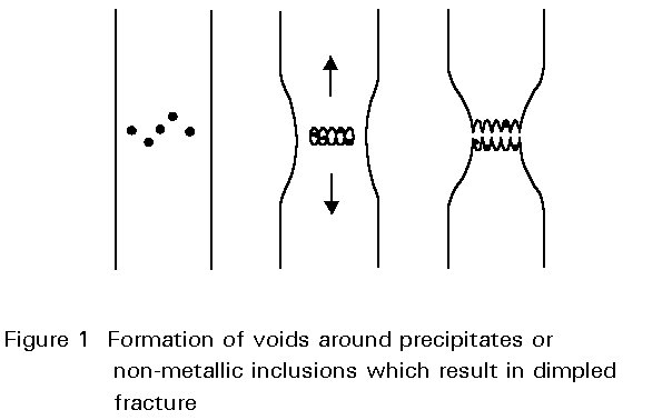
Ductile fracture involves the formation, growth and coalescence of voids. A simple analogy is the fracture of plasticene or putty containing particles of sand. The voids form around precipitates or non-metallic inclusions, Figure 1. The ductility or toughness of the material is basically dependent on the volume fraction of the void nucleating particles, i.e. the proportion of sand in the previous analogy. The amount of deformation prior to rupture and thus the toughness of the material increases with its purity.
The macroscopic orientation of a ductile fracture surface may vary from 90° to 45° to the direction of the applied stress. In thick sections most of the fracture surface tends to be oriented at 90° to the direction of the applied tensile stress. However, ductile fractures commonly have a "shear-tip" near a free boundary as the transverse stresses reduce to zero causing the plane of maximum shear to be at 45° to the direction of the applied stress.
Cleavage fracture occurs in body-centred cubic metals when the maximum principal stress exceeds a critical value, the so-called microscopic cleavage fracture stress s*f.
Certain crystallographic planes of atoms are separated when the stress is sufficiently high to break atomic bonds. Crystallographic planes with low packing densities are preferred as cleavage planes. In steels the preferred change planes are the bee cube planes.
The fracture surface lies perpendicular to the maximum principal stress and appears macroscopically flat and crystalline. When viewed by eye a cleavage fracture usually displays characteristic chevron markings which point back to the origin of the fracture. When brittle fracture occurs in a large structure, such markings can be invaluable in identifying the site of crack initiation. When viewed in the microscope, cleavage cracks can be seen to pass through the grains along preferred crystallographic planes (transgranular cleavage).
If grain boundaries are weakened by precipitates or by the enrichment of foreign atoms, cleavage cracks can also propagate along grain boundaries (intergranular cleavage).
Temperature influences fracture behaviour mainly due to its effect on yield strength and the transition from ductile to cleavage fracture. Figure 2 shows schematically the yield strength and the microscopic cleavage fracture stress as a function of temperature for a ferritic steel. The yield strength falls with increasing temperature, whereas the cleavage fracture stress is hardly influenced. The transition temperature is defined by the intersection between the yield strength and cleavage fracture strength curves. At lower temperatures specimens fail without previous plastic deformation (brittle fracture). Somewhat above the transition temperature, cleavage fracture can still occur due to the effect of deformation induced work hardening. At higher temperatures cleavage is not possible and the fracture becomes fully ductile.
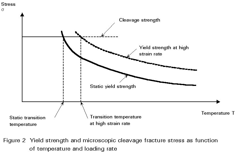
The yield strength rises with increasing loading rate (marked with dashed line in Figure 2) whereas the microscopic cleavage fracture stress shows almost no strain rate dependence. This rise causes the ductile-brittle transition temperature to move to higher values at higher rates of loading. Thus, an increase of loading rate and a reduction of temperature have the same adverse effect on toughness.
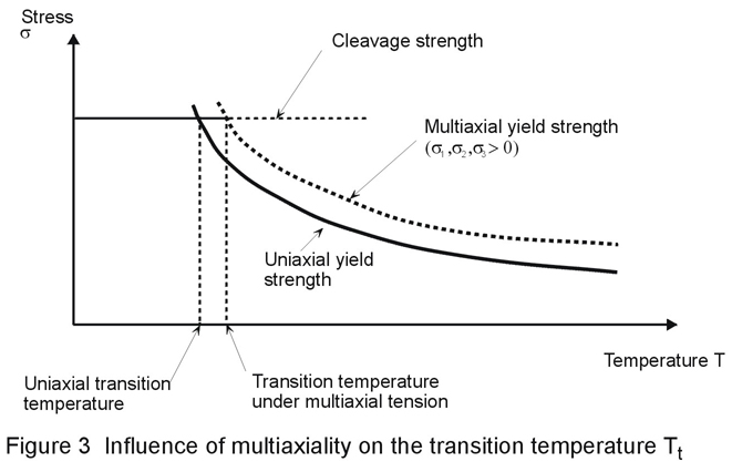
A multi-axial stress state has an important influence on the transition from ductile to cleavage fracture. A triaxial state of stress, in which the three principal stresses s1, s2 and s3 are all positive (but not equal), inhibits or constrains the onset of yielding. Under these conditions, yielding occurs at a higher stress than that observed in a uniaxial or biaxial state of stress. This situation is illustrated in Figure 3 where it can be seen that the transition temperature arising from the intersection of the cleavage and yield strength curves is shifted to a higher temperature, i.e. the metal has become more brittle.
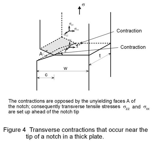
The most familiar situation in which multi-axial states of stress are encountered in steel structures is in association with notches or cracks in thick sections. The stress concentration at the root of the notch gives rise a local region of triaxial stresses even through the applied loading may be uni-directional (Figure 4).
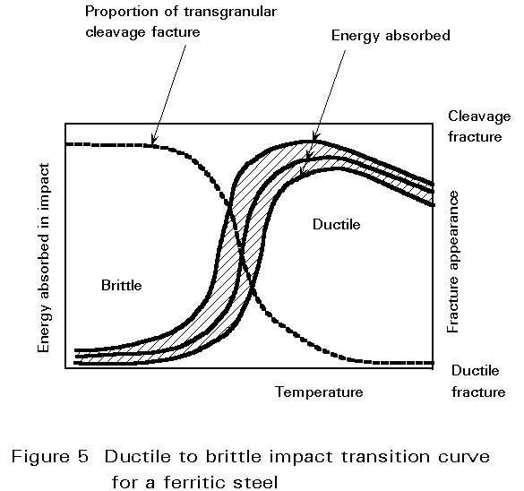
The notched impact bend test is the most common test for the assessment of susceptibility to brittle fracture because it is inexpensive and quickly performed. 10mm square bars with a machined notch, (ISO-V or Charpy specimens), are struck by a calibrated pendulum. The energy absorbed from the swinging pendulum during deformation and fracture of the test specimen is used as a measure of the impact energy. The notch impact energy consists of elastic and plastic deformation work, fracture energy and kinetic energy of the broken pieces.
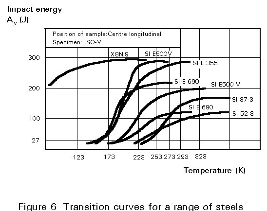
Figures 5 and 6 show the notch impact energy as a function of testing temperature. At low temperatures the failure of ferritic steels occurs by cleavage fracture giving a lustrous crystalline appearance to the fracture surface. At high temperatures failure occurs by ductile fracture after plastic deformation. In the transition range small amounts of ductile fracture are found close to the notch but, due to the elevated stresses near the crack tip, the fracture mechanism changes to cleavage. Throughout the transition range the amount of cleavage fracture becomes less and the notch impact energy rises as the testing temperature increases.
In order to characterise the transition behaviour, a transition temperature is defined as the temperature at which:
The impact energy values obtained show a high amount of scatter in the transition area because here the results depend on the local situation ahead of the crack tip. Beyond this area, scatter becomes less because there is no change of fracture mechanism.
The notched impact bend test gives only a relative measure of toughness. This measure is adequate for defining different grades of toughness in structural steels and for specifying steels for well established conditions of service. For the assessment of known defects and for service situations where there is little experience of brittle fracture susceptibility, a quantitative measure of toughness which can be used by design engineers is provided by fracture mechanics.
Fracture mechanics provides a quantitative description of the resistance of a material to fracture. The fracture toughness is a material property which can be used to predict the behaviour of components containing cracks or sharp notches. The fracture toughness properties are obtained by tests on specimens containing deliberately introduced cracks or notches and subjected to prescribed loading conditions.
Depending on the strength of the material and the thickness of the section, either linear-elastic (LEFM) or elastic-plastic fracture mechanics (EPFM) concepts are applied.
The Linear-Elastic Fracture Mechanics Approach
The stress intensity factor KI describes the intensity of the elastic crack tip stress field in a thick, deeply cracked specimen loaded perpendicular to the crack plane.
KI = Y s ![]() (1)
(1)
where
s
is the nominal stressa is the crack depth
Y is the correction function dependent on the crack and test piece geometry
The critical value of the stress intensity factor for the onset of crack growth is the fracture toughness KIC.
Another material property obtained from linear-elastic fracture mechanics is the energy release rate GI. It indicates how much elastic strain energy becomes free during crack propagation. It is determined according to Equation (2):
GI = p Y2 s2 a / E = K12 / E (2)
where
E is the Young's modulus
Analogous to the stress intensity factor, crack growth occurs when GI reaches a critical value GIc.
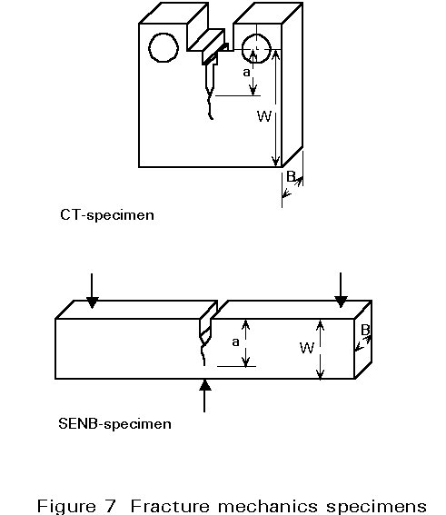
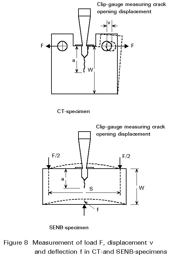
The fracture toughness properties KIc and GIc are determined with fracture mechanics specimens, generally as shown in Figures 7 and 8.
The great value of the fracture toughness parameters KIc and GIc is that once they have been measured for a particular material, Equations (1) and (2) can be used to make quantitative predictions of the size of defect necessary to cause a brittle fracture for a given stress, or the stress which will precipitate a brittle fracture for a defect of known size.
As the designation implies, linear elastic fracture mechanics is applicable to materials which fracture under elastic conditions of loading. The fracture phenomena in high strength quenched and tempered steels are of this type. In lower strength structural steels, extensive plasticity develops at the notch root before failure occurs. This behaviour invalidates many of the assumptions of linear elastic fracture mechanics and makes testing difficult or not meaningful. In such cases elastic-plastic fracture mechanics must be applied.
There are two alternative techniques of elastic-plastic fracture mechanics:
Their essential features are summarised below.
The Elastic-Plastic Fracture Mechanics Approach
A consequence of plasticity developing at the tip of a previously sharp crack is that the crack will blunt and there will be an opening displacement at the position of the original crack tip. This is the crack tip opening displacement (CTOD). As loading continues, the CTOD value increases until eventually a critical value dc is attained at which crack growth occurs.
The critical crack tip opening displacement is a measure of the resistance of the material to fracture, i.e. it is an alternative measurement of fracture toughness.
For materials which exhibit little plasticity prior to failure, the critical CTOD, dc, can be related to the linear elastic fracture toughness parameters KIc and GIc as follows:
KIc2 = E.Gk / (1 - u2) = m.E.sy.dc / (1 - u2)
where
E is Youngs modulus
s
y is the uniaxial yield strengthu
is Poissons ratiom is a constraint factor having a value between 1 and 3 depending on the state of stress at the crack tip.
Another way of taking account of crack tip plasticity is the determination of the J-integral. J is defined as a path-independent line-integral through the material surrounding the crack tip. It is given by:
J = - ![]() (3)
(3)
where
U is the potential energy
B is the specimen thickness
a is the crack length
U =  (4)
(4)
F is the load
Vg is the total displacement
Since the determination of J is difficult, approximate solutions are used in practice.
J = h  (5)
(5)
where
b = w - a
h
= 2 (for SENB-specimens)h
= 2 + 0,522 b/w (for CT-specimens)The critical value of J is a material characteristic and is denoted JIc. For the linear elastic case, JIc is equal to GIc.
Conventional assessment of components is based on a comparison of design resistance with applied actions. Toughness criteria are generally satisfied by the appropriate selection of material quality, as discussed in Lecture 2.5. However there are situations where a more fundamental assessment has to be carried out because of:
Such assessments can be performed by different methods. If the component is small, it may be possible to test it. For large or unique structures, such as bridges or offshore platforms, this method of producing the most realistic data has to be excluded. Tests on representative details of a component may be performed, if the simulation of the real structure is done carefully, e.g. accounting for specific service conditions including the geometry of the structure and discontinuities, loading rate, service temperature and environmental conditions. A typical example of such a test method is the wide plate test, which is discussed below.
Fracture mechanics concepts have been developed to assess the safety of components containing cracks. Depending on the overall behaviour of the component (linear-elastic or elastic-plastic) different methods can be used for failure assessment.
During the last 20 years, large flat tensile specimens, so-called wide plates, have been used to simulate a relatively simple detail of a tension loaded large structure. A main objective of wide plate testing is the evaluation of the deformation and fracture behaviour of a specimen under service conditions. The second reason for this kind of test is the application of test results for the development and checking of failure assessment methods, e.g. fracture mechanics methods.
Wide plate tests require testing facilities with high loading capacities due to the fact that such tests are usually carried out at full thickness. The maximum dimensions of wide plates tested on large test rigs with a load capacity of up to 100MN are as follows:
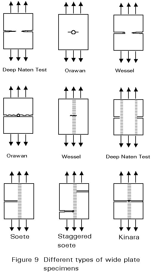
Figure 9 shows different types of specimen containing discontinuities for tests on the base metal or welded joints. The discontinuities may be through-thickness or surface notches or cracks. The configuration of the plate is usually chosen according to the specific structural situation to be assessed.
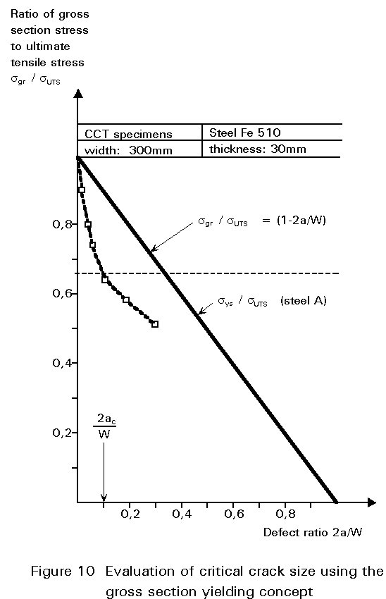
Stress or strain criteria can be used as safety criteria which must be fulfilled to assure the safety of a specific structural element. The production of a given amount of overall strain is in some cases used as the failure criterion. The gross-section-yielding concept requires that gross-section-yielding (GSY) occurs prior to fracture. Based on this concept, wide plates with different crack lengths are tested under similar loading conditions to determine a critical crack length just fulfilling the GSY-criterion. Figure 10 shows the ratio of the maximum gross-section stress in the structure to ultimate tensile strength as a function of the crack length ratio 2a/W of centre-notched wide plates. The upper limit line describes the theoretical maximum stress, if the ultimate tensile strength is reached in the cross-section containing the discontinuity. All test results show lower values than are implied by the theoretical line, resulting from the important influence of toughness in the presence of discontinuities. Only in the case of infinite toughness can the theoretical line be reached. The intersection of the experimentally determined curve and the yield strength line marks the critical crack length ratio 2ac/W. As long as the 2a/W ratio is smaller than the critical ratio, the GSY-criterion is fulfilled. Unfortunately, the critical 2ac/W ratio depends strongly on the dimensions of the crack and the plate, so that different types of cracked components always require a series of specific wide plate tests. This concept is therefore only used if other concepts cannot be applied.
The basis of a fracture mechanics safety analysis is the comparison between the crack driving force in a structure and the fracture toughness of the material evaluated in small scale tests. The application of one of the concepts depends on the overall behaviour of the structure which may be linear-elastic (K-concept) or elastic-plastic (CTOD- or J-Integral-concepts). For a safe structure the crack driving force must be less than the fracture toughness. In general the toughness values of the material are evaluated according to existing standards. The crack driving force can be calculated on the basis of analytical solutions (K-concept), empirical or semi-empirical approaches (CTOD-Design-Curve approach, CEGB-R6-procedures) or using numerical solutions (indirectly: EPRI-handbook, directly: finite-element calculations). The different methods are explained briefly below:
The K-concept can be applied in the case of linear-elastic component behaviour. The crack driving force, the so-called stress intensity factor KI, defined in Section 1.4, has been evaluated for a large range of situations and calculation formulae are for example given in the stress-analysis-of-cracks handbook.
Usually the critical fracture toughness KIc of the material is evaluated according to the ASTM standard E399 or the British Standard BS5447. Brittle failure can be excluded as long as:
KI < KIc
For a given fracture toughness the critical crack length or stress level can be calculated from:
ac = ![]()
s
c =A critical crack length or stress level can be determined using the limit curve of the CTOD-Design-Curve approach for the driving force assessment together with measured values of CTODcrit for the material. The limit curve has been adopted by standards, e.g. the British Standard BS-PD 6493. The latest version of the limit curve is shown in Figure 11 and can be used for:
2a/W £ 0,5 and snet £ sYS.
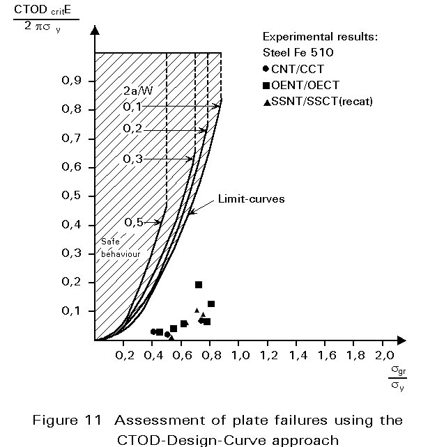
Analysis can only be performed under global elastic conditions (snet £ sYS) although local plastic deformation may occur in front of a crack tip which is accounted for in the CTOD-value of the material.
The CEGB-R6-routines can be used to assess the safety of structures for brittle and ductile component behaviour. The transition from linear-elastic to elastic-plastic behaviour is described by a limit curve in a failure analysis diagram (Figure 12). The ordinate value Kr can be regarded as any of three equivalent ratios of applied crack driving force to material fracture toughness as follows:
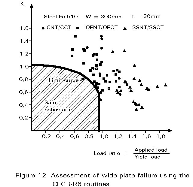
Kr = ![]() =
= ![]()
= ![]()
Other methods are emerging. The Electrical Power Research Institute (EPRI) in New York has used a detailed analysis by finite elements to determine limiting J contour values for standard geometries. Alternatively the J contour values may be obtained by direct finite element analysis of the particular situation.
Preceding sections have described the influence of the micro structure on strength and toughness using metallurgical mechanisms. Chemical and physical metallurgy can change microstructural characteristics so that optimum strength and toughness requirements may be obtained. By combining the various treatments it is possible to achieve a wide range of steel properties (Figure 13):
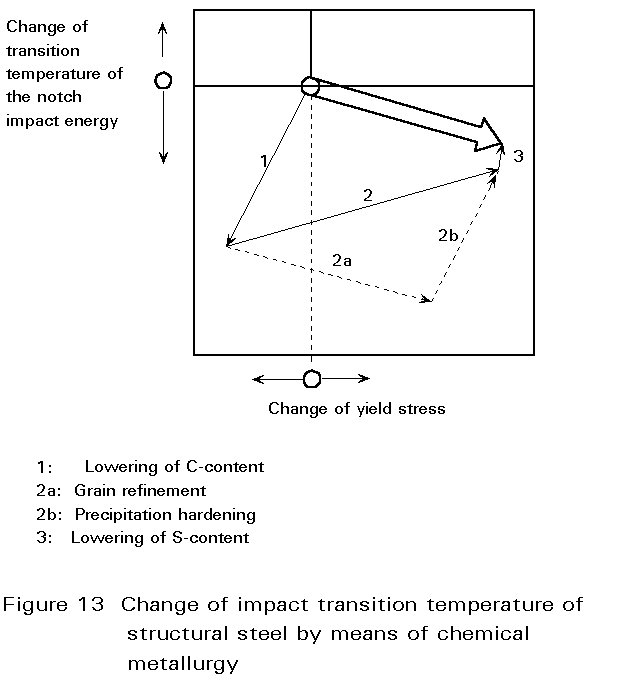
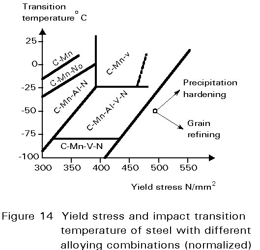
Variation of the chemical composition of a steel by adding alloying elements aims to increase strength and/or increase resistance to brittle fracture. Solid solution hardening generally lowers toughness and is not widely employed. Precipitation hardening also increases strength and decreases toughness. The addition of manganese and nickel produces a small increase in strength due to solution hardening but a more significant reduction is impact transition temperature due to grain refinement (Figure 14). Alloying with the micro-alloying elements Niobium, (Nb) Vanadium (V) and Titanium (Ti) producing carbides and nitrides simultaneously raises strength by precipitation hardening and toughness by grain refinement. Decreasing the content of elements such as S and P improves the degree of purity, which has positive effects on toughness and weldability.
The microstructure of a steel can be greatly affected by heat treatment or forming. Correctly chosen temperature, degree of deformation, time between deformation steps and cooling rate can reduce the grain size and control the state of precipitation, thus raising toughness and strength (Figure 15).
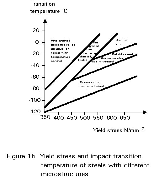
This combination of heat treatment and forming known as thermo-mechanical treatment leads to even better results if micro-alloying elements such as V or Nb are added, causing additional grain refinement with improved toughness and strength properties.
When considering the response of metallic materials to cyclic loading, it is essential to distinguish between components such as machined parts, which are initially free of defects, and those such as castings and welded structures, which inevitably contain pre-existing defects. The fatigue behaviour of these two types of component is quite different. In the former case, the major part of the fatigue life is spent in initiating a crack; such fatigue is 'initiation-controlled'. In the second type of component, cracks are already present and all of the fatigue life is spent in crack propagation; such fatigue is 'propagation-controlled'.
For a given material, the fatigue strength is quite different depending on whether the application is initiation- or propagation-controlled. Also the most appropriate material solution may be quite different depending on the application. For example with initiation-controlled fatigue, the fatigue strength increases with tensile strength and hence it is usually beneficial to utilise high strength materials. On the other hand, with propagation-controlled fatigue, the fatigue resistance may actually decrease if a higher strength material is employed.
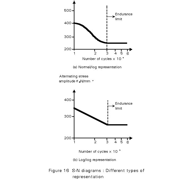
The fundamental diagram in fatigue testing is the Wöhler or S-N-diagram (Figure 16). Specimens are exposed to cyclic loading with a constant amplitude and the number of cycles to fracture is recorded. This parameter is plotted against the corresponding stress amplitude with a double- or semi-logarithmic scale. The diagram is divided into two parts. In the first part, life time increases with decreasing alternating stress amplitude. In the second part for most-ferritic steels the curve becomes horizontal and defines a 'fatigue limit' stress below which failure can never occur. The transition or 'knee' between the two parts of the curve lies between 3 and 10 x 106 cycles, depending on the material. For other alloys, e.g. fcc-metals, which do not show a fatigue limit, an 'endurance limit' is defined as the stress amplitude corresponding to a life of 107 cycles.
One characteristic feature of fatigue properties is the wide scatter of results under constant testing conditions. Therefore 6-10 experiments must be performed for each stress amplitude. The analysis is done by means of statistical evaluation leading to different S-N curves for various life time probabilities (10%, 50%, 90% curves).
During the first 104 stress cycles, although the loading is nominally elastic, dislocation activity occurs in localised areas and leads to the formation of bands of localised plastic deformation known as "persistent slip bands" (PSB).
Crack initiation generally takes place within the persistent slip bands. In the case of pure metals, crack initiation usually occurs at the surface. In commercial quality materials, crack initiation usually occurs at non-metallic inclusions or other impurities which act as microscopic sites of strain concentration.
Once initiated the crack propagates through the first few grains in the direction of maximum shear stress, i.e. at 45° to the normal stress. When the crack has attained a length of a few grain diameters, continued propagation is controlled by the cyclic stress intensity field at the crack tip and the crack path becomes oriented at 90° to the maximum principal stress direction. Although the major part of the fatigue life is spent in crack initiation, this is not apparent from examination of the fracture surface where only the final propagation stage can be seen.
The relationships between initiation-controlled fatigue strength and other parameters are complex and sometimes only known qualitatively. Nevertheless they are of great importance for material selection and dimensioning of structural parts. Therefore a number of different parameters are discussed below with respect to their influence on fatigue properties.
The S-N diagram characterises material behaviour under single-amplitude loading. For weight-saving constructions exposed to complex stresses, the parameters determined by such tests are not sufficient.
For testing under realistic conditions, an analysis of the actual stresses has to be obtained. For that purpose the sequence and duration of different stress levels, as well as their rise or fall, are recorded. This stress-time function is either reproduced under laboratory conditions, or special testing programmes are calculated from these data and used in experiments. Results obtained by this method cannot be transferred to different materials and loading conditions.
The fundamental method of life time cumulative damage prediction was formulated by Miner. The damage from each cycle at a certain stress level is defined as the reciprocal value of the number of cycles to fracture (1/Ni). Fracture occurs when the sum of cycles at each level (ni) related to the number of cycles to failure (Ni) is equal to unity. The mathematical expression is:
![]()
Since this is a very simple equation, results are widely scattered. In reality the values form a Gaussion distribution with a maximum around 1. To guarantee safe construction, calculations are made with factors smaller than 1 and stresses below their maximum values. Furthermore it is possible to take the effects of different loading levels into account with respect to their number, maximum stress and sequence.
Steel castings, rough forgings and welded structures invariably contain surface imperfections which behave as minute crack-like defects which effectively eliminate the crack-initiation stage in fatigue. Consequently the whole of the fatigue life is concerned with crack propagation. The rate of crack advance is determined by the cyclic stress intensity D Kr which is the cyclic equivalent of the stress intensity factor KI defined in Section 1.5.
DKI = Y Ds ![]()
where
Ds
is the cyclic stress rangea is the crack depth
Y is the correction function dependent on the crack and test piece geometry.
The rate of crack propagation is then given by the following relationship which is known as Paris' Law:
![]() = C DKIm
= C DKIm
N = Number of cycles
C is a material constant which is inversely proportional to Young's modulus E. The power m has a value of about 3 for most metallic materials.
The advantage of the fracture mechanics description of crack propagation is that the rate equation can be integrated to determine the number of cycles required for a crack to propagate from some initial length ai to same final length af. Thus for m = 3;
Nf = 2 (1/ai½ - 1/af½ ) / (CY3Ds3p3/2)
ai may be a known crack size or an NDT limit, af may be a critical defect size for unstable fracture or a component dimension such as the wall thickness of a vessel.
In the above equation for the fatigue life, the constant C is dependent on the type of material but is not sensitive to variations in microstructure or strength level. Consequently, for a given cyclic stress range, Ds, the fatigue life is independant of the strength of the material. If, however, the stress range increases in proportion to the material yield strength, then the fatigue life will be less for the higher strength material. For example, a two-fold increase in stress range produces almost a ten-fold reduction in fatigue life. This is a major constraint on the utilisation of higher strength structural steels for fatigue dominated applications.
The fatigue behaviour of welded joints is propagation-controlled. However it is impracticable to apply a fracture mechanics analysis because the initial defect size cannot be evaluated and the cyclic stress range is amplified by local stress concentration effects associated with the weld profile. Instead the fatigue strength is determined experimentally for the range of weld types and welding processes which are commonly employed in welded structures. This data is presented as a series of S-N curves for different weld classifications as shown in Figure 16.
The fatigue strength of welded joints is not sensitive to the strength of the parent plate. Consequently, as explained previously, it is difficult to take full advantage of higher strength steels in welded structures where there is significant exposure to cyclic loading.
× Reducing temperature
× Increasing strain rate
× Multi-axial tension
× Geometric discontinuities causing stress concentrations.
APPENDIX 1
Fracture toughness values of different materials
|
Material |
Kc (MNm-3/2) |
Material |
Kc (MNm-3/2) |
|
Ductile metals, e.g. Cu |
200 |
cast iron |
15 |
|
Grade Fe430B structural steel (room temperature) |
140 |
glass reinforced plastic |
40 12 |
|
Grade Fe 430B structural steel (-100° C) |
40 |
||
|
Pressure vessel steels |
170 |