ESDEP WG 16
STRUCTURAL SYSTEMS: REFURBISHMENT
To demonstrate the means by which existing bridges may be assessed and, where necessary, strengthened.
None.
Lecture 15B.2 Actions on Bridges
A majority of existing steel bridges for road and rail are riveted structures built in the last century.
Many of these old bridges have been repaired or strengthened several times following damage in the World Wars or due to changes of service requirements. The safety of these bridges for modern traffic loads throughout their remaining service life needs to be assessed.
A classical method for the assessment of the remaining fatigue safety of existing railway bridges is given. This method is based on the procedure given in the Standards of the German Railways. It is noted that the S-N lines referred to in this method do not comply with the S-N lines given in Eurocode 3. Also the safety assumptions used in this method are different to those specified in Eurocode 3. The method may, however, be easily transferred into the Eurocode system. The method is illustrated by a numerical example. Similar principles apply to highway bridges.
General methods for strengthening bridges are outlined and a case study is presented.
The nature of bridge behaviour is such that the structure should be subject to regular inspection and maintenance. Old steel bridges that are subjected to growing traffic density and traffic loads may need a general safety check to evaluate them to determine their residual safety and remaining service life. This may include:
Methods for evaluating the remaining service life of existing structures are becoming increasingly important as the number of structures exceeding their design life is growing exponentially. This growth is related to the bridge construction boom which began over one hundred years ago. Few structures need to be replaced when they reach their design life, because the design life was not defined scientifically in the past. Most structures are able to endure fatigue loading well beyond their original design life.
The design life is that period for which a bridge is required to perform safely with an acceptable probability that it will not require repair.
Generally, little is known of previous loading, structural modifications or possible crack location in an existing bridge. Starting with simple conservative assumptions and proceedings in steps, an acceptable decision can be taken regarding the safety of the structure.
In the following a classical method for the assessment of the remaining fatigue safety of existing railway bridges is given. This method is based on the procedure given in the Standards of the German Railways.
It is noted that the S-N lines referred to in this method do not comply with the S-N lines given in Eurocode 3. Also, the safety assumptions used in this method are different to those specified in Eurocode 3. The method may, however, be easily transferred into the Eurocode system in due course.
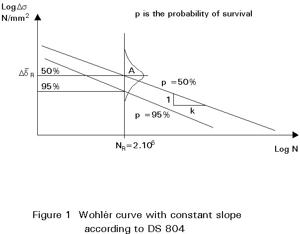
A first step in evaluating the remaining service life of an existing steel railway bridge is to assess their fatigue life with Wöhler curves.
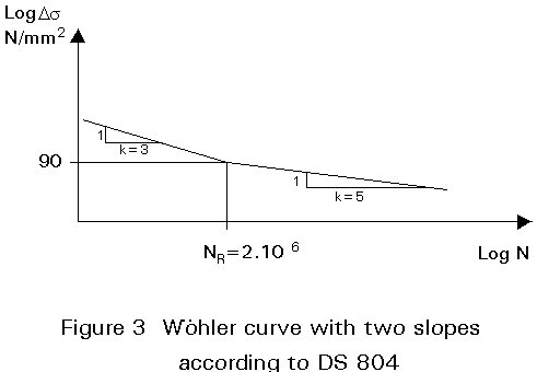
Fatigue failure occurs in elements subjected to variable loads at values significantly below those that would cause failure under static conditions. The first systematic studies on fatigue were carried out by Wöhler. The expression linking the number of cycles N and the stress range Ds = smax-smin (the algebraic difference between the two extremes of a stress cycle) can be plotted on a logarithmic scale as a straight line. The line is known as the Wöhler curve (or the S-N curve). The fatigue strength is defined by a series of Wöhler curves, each applying to a typical detail category (the designation given to a particular welded or bolted detail). These curves are obtained experimentally from a great number of tests. Generally the linear part of the Wöhler curve is defined by:
Ni = (DsR /Dsi)k . NR (1)
or Ni = C Dsik
where:
C = NR DsRk (2)
or log Ni = log (NR DsRk) - k log Dsi (3)
where:
Ds
1, Ds2 are individual stress ranges in a design spectrumni are the number of applied repetitions of damaging stress ranges Dsi
Ni are the number of stress range repetitions Ds1, Ds2.... bringing about failure, corresponding to n1, n2 .... repetitions of applied stress cycles.
NR = 2 ´ 106 cycles
Ds
R = fatigue strength at NR cyclesk is the slope of the curve.
There are different forms of Wöhler curves that may be used for damage calculations:

The following points should be noted:
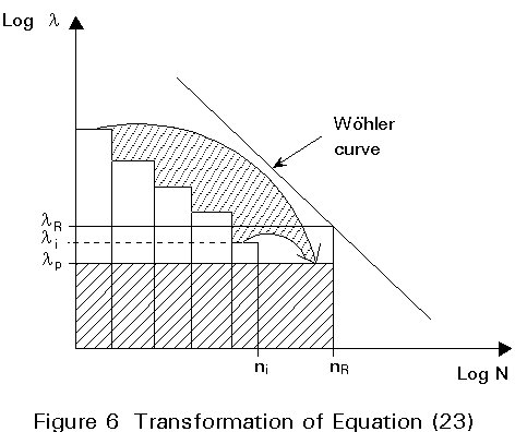
The cumulative damage induced by different loading patterns acting on a structure is given by:
S = ![]() (4)
(4)
Equation (4) can be transformed (Figure 4)
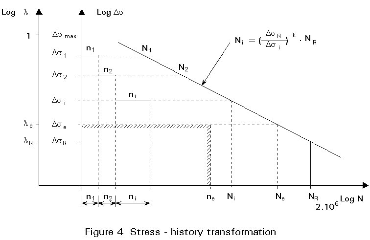
![]() (5)
(5)
From Equation (1) for a linear part of the S-N curve
Ni = NR DsRk / Dsik = C / Dsik (6)
Ne = NR DsRk / Dsek = C / Dsek (7)
(e = equivalent)
where C is a constant value defined by N = 2 ´ 106
Substituting Equations (6) and (7) into Equation (5) gives:
![]() (8)
(8)
and finally:
S
ni Dsik = ne Dsek (9)Stress ranges can be related to the value
Ds
UIC = (max sUIC - min sUIC)where sUIC are the stresses resulting from the standard UIC loading, with appropriate allowance for dynamic effects, as discussed below.
If l = Dsi /DsUIC then
S
ni Dlik = ne . lek (10)Mathematically the relation expresses the equivalence between the different areas in Figure 4.
The dynamic effect of a moving train is generally expressed as a percentage of the static live load. For instance the International Union of Railways (UIC) and the German Standard DS 805 [2] gives the following expression for the dynamic coefficient:
1 + r (11)
where r = a1 r¢ + a2 r² r < 1 (12)
r¢ refers to an intact rail
r² takes into account the imperfections of the rail
The values a1 and a2 are:
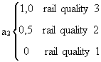
The German Standard [2] gives the following definitions for the rail quality:
Quality 3 - Imperfections of 2 mm depth on 1000 mm length; usually before 1930, or when the speed v < 80 km/h
Quality 2 - Imperfections of 1 mm depth on 1000 mm length of the rail; for speed 80 < v < 140 km/h
Quality 1 - without rail imperfections; for v > 140 km/h
The values of r¢ and r² are given in Tables 1 and 2.
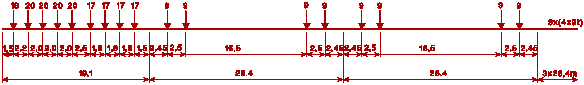
The UIC 71 loading represents the static effect of normal rail traffic on the track, as shown in Figure 5.
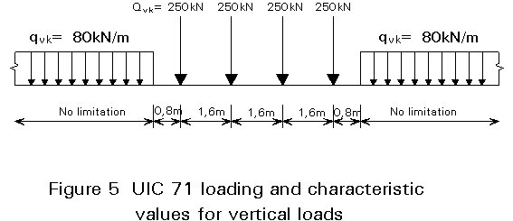
Taking into account the dynamic effects resulting from the movement of vehicles at speed, the equivalent load can be calculated from the static loads, multiplied by a dynamic factor as follows:
|
{1,67 |
0 £ L £ 3,61m |
|
{1,44 / (ÖLf - 0,2) + 0,82 |
3,61 £ L £ 65m |
(13) |
|
{1,00 |
65m £ L |
The values of the characteristic length Lf can be taken from Table 3.
According to DS 805 [2] the definition of an existing structure is one which is more than 10 years old. The main steps in evaluating the safety of existing bridges are as follows:
S =
where
(14)
Ni =
(15)
where DsR is the design stress range value for NR = 2 ´ 106 cycles, obtained by applying a safety coefficient
DsR = D
/gR (gR = 1,65)
D
Dsi is the stress range value for Ni cycles
Dsuic = max suic - min suic
and Dsi / Dsuic = li; D
The following points should be noted:
1. The introduction of these values enables the ratio li to be tabulated:
li = Dsi / Dsuic = [(1 + r)/f].(DMi / DMuic) (17)
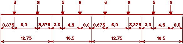
2. For a simply supported girder in Table 3 (Case 5) the bending moments produced by the UIC 71 loading pattern are given in Table 4.
Ni = [lR/li]k NR(18)
Sp = Si [(nilik)/(NRlRk)] = [1/NRlRk].Si nilik (19)
ZTm = 365 Tn Sj Nj (20)
For the evaluation of the fatigue safety of the structure it is necessary to reconsider the traffic in the past. This a difficult problem; analysing all the traffic for a certain period it is possible to typify the trains. Such train types of fatigue according to the DS 805, are given in Table 5; the corresponding values for the related damage lTj for each train are shown in Table 6.
STm = 365/(NRlRk) . Tn Sj NjnlTjk (21)
Sp = 365/(NRlRk) . Smn=1 Tn Sj Njn(lTjn)k (22)
gt,p = [1/Sp]1/k ³ 1 (23)
[1/Sp]1/k = [NR lRk/Sni lik]1/k
[1/Sp]1/k = lR[NR /S ni lik]1/k
With S ni lik = NR lpk
gives 1/lpk= NR /S ni lik
and finally [1/Sp]1/k = lR/lp ³ 1
The ratio of the two values depends on the adopted safety concept; the smaller lp is in comparison to lR, the greater the safety.
1. Structures or elements, for which the condition
gtk . Sp £ 1 (24)
is satisfied and there are no cracks. These may be regarded as sufficiently safe against fatigue failure.
In the relation above gt is a split coefficient depending on the age of the structure at the moment of calculation:
gt = gR,t . gS,t (25)
gR,t =
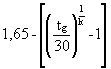
gS,t = 1,15
tg - age of the structure.
2. If:
1,0 £ gtk . Sp < 1,1 (26)
and no cracks are found which need immediate action, then at the next inspection special attention must be paid to these elements.
3. If:
1,1 £ gtk . Sp < 1,2 (27)
immediate special inspection must be ordered and repeated after 3 years; special attention must be paid to the cracks and their rate of growth.
4. When:
gtk . Sp ³ 1,2 (28)
immediate special inspection must be ordered and repeated every year. Other maintenance measures must be taken; special attention must be paid to the cracks.
This process is illustrated in the example on page 24.
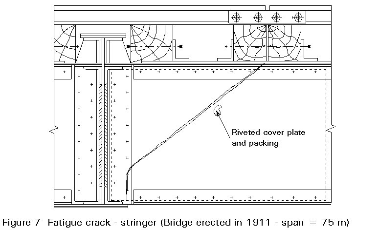
It should be noted that it is not possible to prevent all failures, but if major collapses are to be prevented, the lessons from previous failures must be learned. Figure 7 shows a fatigue crack which appeared in a stringer of a bridge build in 1911 with a span of 75 m. This failure was caused by an imperfect rail joint.
During service, bridges are subject to wear; in addition, the initial volume of traffic has increased, particularly over the last 50 years. Many bridges therefore require strengthening.
It is first necessary to assess the condition of the bridge, and then, if necessary, to have a scheme for strengthening. The inspection should consider:
(a) the age of the bridge and any repairs;
(b) the extent and location of any defects: cracks, local deformations, corrosion, etc.
(c) in situ data on steel grade, stress and strain at different points, etc.
The assessment should include a feasibility study to demonstrate the cost-benefit of strengthening. It must be emphasised that strengthening may extend the life of a bridge by about 20-40 years. It does not create a new bridge, and hence is only a realistic proposition if the cost is less than 40% of a replacement bridge.
This is used to overcome local defects and involves fitting additional elements. There are two possibilities:
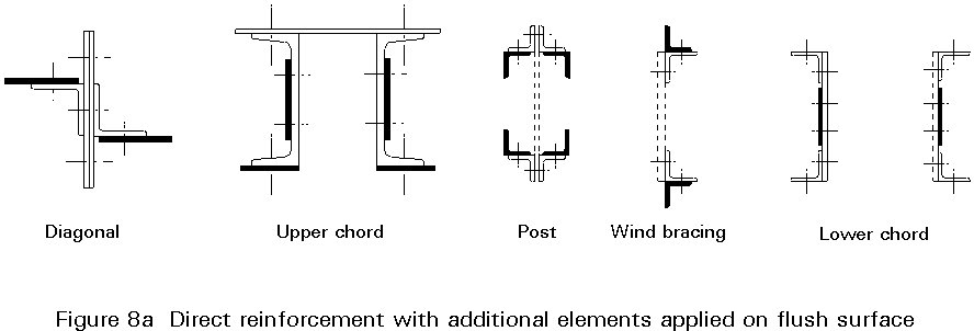
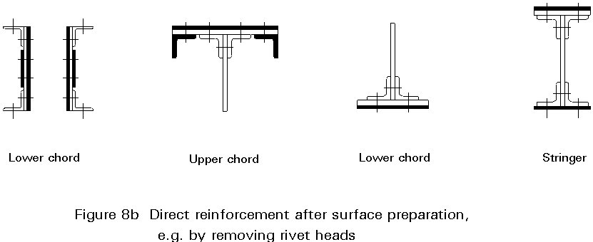
In this case independent elements are inserted within the structure. There are many types. Some may allow initial prestressing forces, thereby increasing the efficiency of the reinforcement.
The principal methods of providing indirect strengthening are:
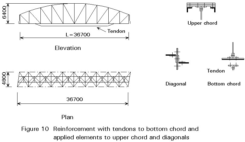
Strengthening with tendons
The tendons can be a simple bar or a built-up section placed at the level of tension chord; it may be prestressed and is typically used to strengthen bridges of lattice girder or truss construction (Figure 9 and Figure 10).

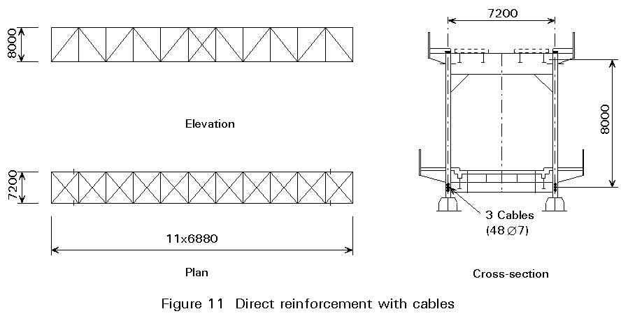
Strengthening by cables
Prestressed cables can be used in a similar way, fitted alongside or within existing tension elements.
For the example shown in Figure 11, three cables were introduced at the centre of the lower tension chord; as a result of the prestressing force in the cables this chord became almost completely unstressed under dead load. To increase the load carrying resistance of the complete trusses, the upper chord and the lateral diagonals were also reinforced but using direct strengthening measures.
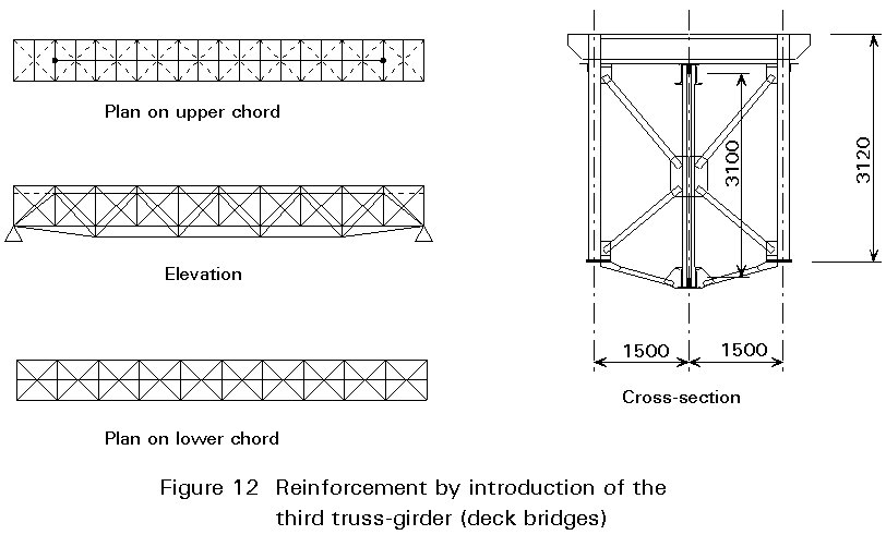
Reinforcement by additional trusses
Deck bridges can be strengthened by adding a third main girder connected to the existing structure in order to increases its load carrying resistance (Figure 12).
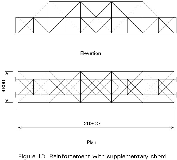
Increasing the effective depth
Reinforcement by a new chord connected to that existing by a triangulated arrangement of members, effectively increasing the height of the main truss (Figure 13).
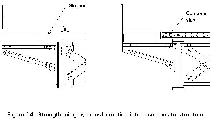
Strengthening plate girders by transformation into composite sections
The concrete slab replaces the sleepers; this maintains the original constructional depth. The concrete slab will act as an integral part of the compression flanges of the stringers and floor beams, Figure 14.
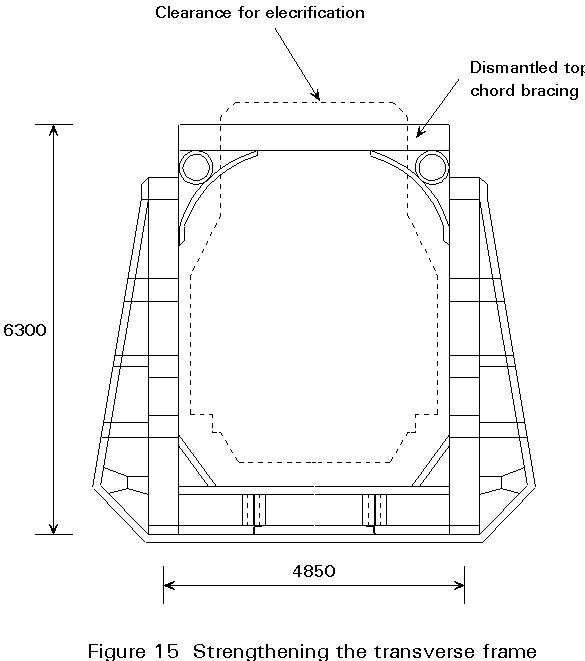
Reinforcement of the transverse frame
For semi - through trusses and through trusses where the wind-bracing has been removed during electrification of the line, it may be necessary to increase the rigidity of the transverse frame. For this purpose a tendon is introduced into the cross-section (Figure 15).
The bridge over the Danube at Cernavoda (Figure 16) was built in 1895. Since then, especially after World War II, traffic and hence live load have grown in the structure to a level which endangered its safety. As a result major strengthening was necessary. This work had to be completed without interrupting the traffic.

Many of the methods outline above were used (Figure 17).

The bottom chords were strengthened by adding a third web connected by riveted diaphragms. The stringers were replaced.
For strengthening the cross girders, a pretensioned girder was used.
For the compression diagonals direct strengthening was achieved by fitting additional plates. The tension diagonals were strengthened with tendons.
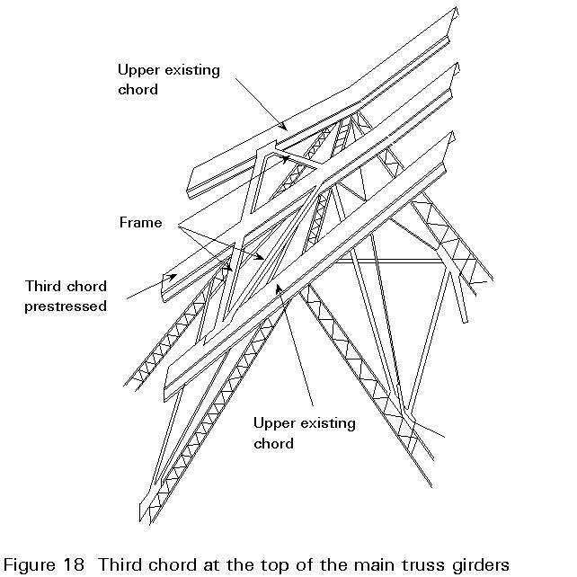
The most difficult problem was strengthening of the upper chord. It was finally decided to introduce a third chord located between the existing ones (Figure 18). In order to relieve the existing chords of the stresses produced by dead load, the third chord, representing 45% of the existing sections, was prestressed.
A total of 4.000 tonnes of steel was used. Strengthening was completed in 1967. After 25 years of subsequent use the bridge has presented no special maintenance problems.
[1] "Bestehende Eisenbahnbrücken. Bewertung der Tragsicherheit und konstruktive Hinweise" DS 805, Deutsche Bundesbahn Mai 1991.
Table 1 Values of the Coefficient
r ' [2]|
v
[km/h]
l [m] |
10 |
20 |
30 |
40 |
50 |
60 |
70 |
80 |
90 |
100 |
110 |
120 |
140 |
160 |
180 |
|
2 |
0,0177 |
0,0360 |
0,0549 |
0,0746 |
0,0951 |
0,1163 |
0,1383 |
0,1612 |
0,1851 |
0,2099 |
0,2357 |
0,2625 |
0,3196 |
0,3815 |
0,4483 |
|
5 |
0,0177 |
0,0360 |
0,0549 |
0,0746 |
0,0951 |
0,1163 |
0,1383 |
0,1612 |
0,1851 |
0,2099 |
0,2357 |
0,2625 |
0,3196 |
0,3815 |
0,4483 |
|
7 |
0,0177 |
0,0360 |
0,0549 |
0,0746 |
0,0951 |
0,1163 |
0,1383 |
0,1612 |
0,1851 |
0,2099 |
0,2357 |
0,2625 |
0,3196 |
0,3815 |
0,4483 |
|
10 |
0,0177 |
0,0360 |
0,0549 |
0,0746 |
0,0951 |
0,1163 |
0,1383 |
0,1612 |
0,1851 |
0,2099 |
0,2357 |
0,2625 |
0,3196 |
0,3815 |
0,4483 |
|
15 |
0,0177 |
0,0360 |
0,0549 |
0,0746 |
0,0951 |
0,1163 |
0,1383 |
0,1612 |
0,1851 |
0,2099 |
0,2357 |
0,2625 |
0,3196 |
0,3815 |
0,4483 |
|
20 |
0,0177 |
0,0360 |
0,0549 |
0,0746 |
0,0951 |
0,1163 |
0,1383 |
0,1612 |
0,1851 |
0,2099 |
0,2357 |
0,2625 |
0,3196 |
0,3815 |
0,4483 |
|
30 |
0,0149 |
0,0303 |
0,0462 |
0,0625 |
0,0794 |
0,0968 |
0,1148 |
0,1334 |
0,1526 |
0,1725 |
0,1930 |
0,2142 |
0,2589 |
0,3067 |
0,3579 |
|
40 |
0,0133 |
0,0269 |
0,0409 |
0,0552 |
0,0700 |
0,0852 |
0,1008 |
0,1169 |
0,1335 |
0,1505 |
0,1681 |
0,1862 |
0,2240 |
0,2642 |
0,3069 |
|
50 |
0,0121 |
0,0245 |
0,0372 |
0,0502 |
0,0635 |
0,0772 |
0,0913 |
0,1057 |
0,1205 |
0,1357 |
0,1513 |
0,1673 |
0,2007 |
0,2360 |
0,2733 |
|
70 |
0,0105 |
0,0213 |
0,0323 |
0,0435 |
0,0549 |
0,0667 |
0,0786 |
0,0909 |
0,1034 |
0,1163 |
0,1294 |
0,1428 |
0,1706 |
0,1998 |
0,2304 |
|
100 |
0,0091 |
0,0183 |
0,0278 |
0,0374 |
0,0472 |
0,0571 |
0,0673 |
0,0776 |
0,0882 |
0,0990 |
0,1100 |
0,1212 |
0,1442 |
0,1683 |
0,1933 |
|
120 |
0,0084 |
0,0170 |
0,0257 |
0,0346 |
0,0436 |
0,0528 |
0,0622 |
0,0717 |
0,0814 |
0,0912 |
0,1013 |
0,1115 |
0,1325 |
0,1544 |
0,1771 |
Table 2 Values of the Coefficient
r ' [2]|
v [km/h] l [m] |
10 | 20 | 30 | 40 | 50 | 60 | 70 | 80 | 90 | 100 | 110 | 120 | 140 | 160 | 180 |
|
2 |
0,0673 |
0,1345 |
0,2018 |
0,2690 |
0,3363 |
0,4055 |
0,4708 |
0,5380 |
0,5380 |
0,5380 |
0,5380 |
0,5380 |
0,5380 |
0,5380 |
0,5380 |
|
5 |
0,0545 |
0,1090 |
0,1635 |
0,2181 |
0,2726 |
0,3271 |
0,3816 |
0,4361 |
0,4361 |
0,4361 |
0,4361 |
0,4361 |
0,4361 |
0,4361 |
0,4361 |
|
7 |
0,0429 |
0,0858 |
0,1287 |
0,1715 |
0,2144 |
0,2573 |
0,3002 |
0,3431 |
0,3431 |
0,3431 |
0,3431 |
0,3431 |
0,3431 |
0,3431 |
0,3431 |
|
10 |
0,0258 |
0,0515 |
0,773 |
0,1030 |
0,1288 |
0,1545 |
0,1603 |
0,2060 |
0,2060 |
0,2060 |
0,2060 |
0,2060 |
0,2060 |
0,2060 |
0,2060 |
|
15 |
0,0074 |
0,0148 |
0,0221 |
0,0295 |
0,0369 |
0,0443 |
0,0516 |
0,0590 |
0,0590 |
0,0590 |
0,0590 |
0,0590 |
0,0590 |
0,0590 |
0,0590 |
|
20 |
0,0013 |
0,0026 |
0,0038 |
0,0051 |
0,0064 |
0,0077 |
0,0090 |
0,0103 |
0,0103 |
0,0103 |
0,0103 |
0,0103 |
0,0103 |
0,0103 |
0,0103 |
|
30 |
0,0012 |
0,0024 |
0,0036 |
0,0048 |
0,0060 |
0,0072 |
0,0084 |
0,0095 |
0,0095 |
0,0095 |
0,0095 |
0,0095 |
0,0095 |
0,0095 |
0,0095 |
|
40 |
0,0004 |
0,0007 |
0,0011 |
0,0015 |
0,0019 |
0,0022 |
0,0026 |
0,0030 |
0,0030 |
0,0030 |
0,0030 |
0,0030 |
0,0030 |
0,0030 |
0,0030 |
|
50 |
0,0001 |
0,0001 |
0,0002 |
0,0002 |
0,0003 |
0,0003 |
0,0004 |
0,0004 |
0,0004 |
0,0004 |
0,0004 |
0,0004 |
0,0004 |
0,0004 |
0,0004 |
|
70 |
0,0000 |
0,0000 |
0,0000 |
0,0000 |
0,0000 |
0,0000 |
0,0000 |
0,0000 |
0,0000 |
0,0000 |
0,0000 |
0,0000 |
0,0000 |
0,0000 |
0,0000 |
|
100 |
0,0000 |
0,0000 |
0,0000 |
0,0000 |
0,0000 |
0,0000 |
0,0000 |
0,0000 |
0,0000 |
0,0000 |
0,0000 |
0,0000 |
0,0000 |
0,0000 |
0,0000 |
|
120 |
0,0000 |
0,0000 |
0,0000 |
0,0000 |
0,0000 |
0,0000 |
0,0000 |
0,0000 |
0,0000 |
0,0000 |
0,0000 |
0,0000 |
0,0000 |
0,0000 |
0,0000 |
Table 3 Definitions of characteristic lengths for fatigue calculations
|
Case |
Structural Element |
Characteristic Length L f |
|
DECK PLATE (Steel) closed deck with ballast bed (orthotropic deck plate) (for local stresses) |
||
|
1
|
Deck with longitudinal and cross ribs |
|
|
1.1 Deck plate (for both directions) |
3 ´ cross girder spacing |
|
|
1.2 Longitudinal ribs (including small cantilevers up to 0,50m)(*) |
3 ´ cross girder spacing |
|
|
1.3 Cross girders, end cross girders |
2 ´ length of cross girders |
|
|
2
|
Deck plate with cross girders only |
|
|
2.1 Deck plate (for both directions) |
2 ´ cross girder spacing + 3 m |
|
|
2.2 Cross girders, end cross girders |
2 ´ length of cross girders |
|
|
DECK PLATE (Steel) open deck without ballast bed (for local stresses) |
||
|
3
|
3.1 Rail bearers - as an element of a grillage - simply supported |
3 ´ cross girder spacingcross girder spacing + 3 m |
|
3.2 Cantilever of rail bearer |
the characteristic length leads to f 3 = 2,0 |
|
|
3.3 Cross girders, end cross girders |
2 ´ length of cross girders |
|
|
DECK PLATE WITH BALLAST BED (structural concrete) (for local and transverse stresses) |
||
|
4
|
4.1 Deck plates as part of box girders or upper flange of main beam |
|
|
- spanning transversely to the main girders |
3 ´ span of deck plate |
|
|
- spanning in the longitudinal direction |
3 ´ span of deck plate or characteristic length of main girder; whichever is the lesser |
|
|
- transverse cantilevers supporting railway loading |
see footnote (**) |
|
|
4.2 Deck plate continuous over cross girders (in main-girder direction) |
2 ´ span of deck plate in the longitudinal direction |
|
|
4.3 Deck plate for trough bridges: |
|
|
|
- spanning perpendicular to the main girders |
span of deck plate |
|
|
- spanning in the longitudinal direction |
2 ´ span of deck plate or characteristic length of main girders; whichever is the lesser |
|
|
4.4 Deck slabs spanning transversely between steel beams embedded in concrete |
2 ´ characteristic length in the longitudinal direction |
|
|
MAIN GIRDER ELEMENTS |
||
|
5
|
5.1 Simply supported girders and slabs (including steel girders embedded in concrete) |
Span in main girder direction |
|
5.2 Girders and slabs continuous over n spans with: |
L f = k . Lm, at least max. Li (i=1,....,n) |
|
|
Lm = |
|
|
*
In general all cantilevers greater than 0,50 m and supporting railway loads need a special study.(**)
These cantilevers need a special study.Table 4 Maximum bending moments produced in a simply supported girder by the UIC 71 loading
|
L (m) |
Mmax (kN.m) |
L (m) |
Mmax (kN.m) |
L (m) |
Mmax (kN.m) |
|
1,0 1,2 1,4 1,6 1,8 2,0 2,2 2,4 2,6 2,8 3,0 3,2 3,4 3,6 3,8 4,0 4,2 4,4 4,6 4,8 5,0 |
62,5 75,0 87,5 100,0 112,7 125,8 139,3 153,2 167,5 182,2 197,3 212,8 241,2 275,0 312,5 350,0 387,5 425,0 462,5 500,0 537,7 |
6 7 8 9 10 11 12 13 14 15 16 17 18 19 20 22 24 26 28 30 32 |
732,2 974,2 1251 1543 1855 2187 2539 2911 3303 3715 4147 4599 5071 5563 6075 7159 8323 9567 10890 12300 13780 |
34 36 38 40 42 44 46 48 50 52 54 56 58 60 65 70 75 80 85 90 100 |
15340 16990 18710 20520 22400 24360 26410 28530 30740 33020 35380 37830 40350 42960 49820 57180 65040 73400 82260 91620 111800 |
Table 5 Historical types of trains for fatigue analysis [1]
Type 2.1 (1876-1890) S P = 126,5 t L = 64,04 m

Type 2.2 (1876-1890) S P = 249 t L = 77,18 m

Type 3.1 (1891-1905) S P = 166 t L = 76,15 m
Type 3.2 (1891-1905) S P = 325 t L = 76,98 m

Type 4.1 (1906-1920) S P = 205,1 t L = 95,02 m
Type 6.1 (1936-1950) S P = 294 t L = 98,78 m

Type 6.2 (1936-1950) S P = 478 t L = 171,14 m

Type 6.3 (1936-1950) S P = 732 t L = 271,9 m

Type 7.1 (1951-1965) S P = 52 t L = 46,5 m
Type 7.2 (1951-1965) S P = 346 t L = 151,1 m
Type 7.3 (1951-1965) S P = 406 t L = 177,5 m
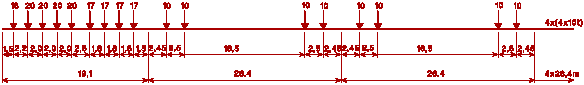
Table 6 lTj - for fatigue trains-past (k = 5) [2]
|
Period
|
Train j
|
Span l [m] |
|||||||||
|
2 |
3 |
5 |
7 |
10 |
15 |
20 |
25 |
50 |
100 |
||
|
1 |
1 2 |
|
|
|
|
|
|
|
|
|
|
|
2 |
1 2 |
0,637 0,709 |
0,595 0,653 |
0,423 0,523 |
0,411 0,515 |
0,364 0,445 |
0,577 0,577 |
0,370 0,412 |
0,298 0,335 |
0,277 0,358 |
0,116 0,197 |
|
3 |
1 2 |
0,721 0,884 |
0,612 0,823 |
0,466 0,529 |
0,464 0,515 |
0,404 0,445 |
0,635 0,577 |
0,453 0,412 |
0,335 0,335 |
0,325 0,374 |
0,134 0,224 |
|
4 |
1 2 3 |
0,753 0,938 0,891 |
0,685 0,798 0,810 |
0,477 0,580 0,484 |
0,463 0,577 0,465 |
0,445 0,549 0,446 |
0,692 0,756 0,635 |
0,494 0,535 0,453 |
0,410 0,447 0,373 |
0,358 0,423 0,390 |
0,155 0,189 0,218 |
|
5 |
1 2 3 |
1,116 1,117 1,104 |
0,891 0,911 1,019 |
0,657 0,666 0,748 |
0,668 0,609 0,748 |
0,647 0,589 0,744 |
0,981 0,813 1,043 |
0,700 0,618 0,701 |
0,596 0,522 0,560 |
0,569 0,537 0,537 |
0,247 0,229 0,245 |
|
6 |
1 2 3 |
1,090 1,148 1,071 |
0,869 0,888 1,010 |
0,672 0,699 0,814 |
0,671 0,692 0,832 |
0,687 0,699 0,813 |
0,981 0,983 1,156 |
0,741 0,741 0,782 |
0,596 0,596 0,634 |
0,569 0,569 0,602 |
0,229 0,239 0,253 |
|
7 |
1 2 3 4 |
0,427 1,134 1,148 1,385 |
0,411 0,810 0,843 1,264 |
0,252 0,658 0,660 0,883 |
0,185 0,673 0,674 0,782 |
0,125 0,689 0,691 0,777 |
0,174 1,040 1,043 1,100 |
0,124 0,782 0,783 0,743 |
0,112 0,634 0,634 0,634 |
0,114 0,602 0,602 0,667 |
0,053 0,232 0,237 0,310 |
|
8 |
1 2 3 4 |
0,427 1,068 1,193 1,413 |
0,411 1,016 0,981 1,355 |
0,252 0,515 0,670 0,805 |
0,185 0,447 0,643 0,633 |
0,125 0,416 0,582 0,499 |
0,174 0,592 0,722 0,676 |
0,124 0,415 0,541 0,468 |
0,112 0,373 0,450 0,379 |
0,114 0,325 0,439 0,409 |
0,053 0,134 0,184 0,211 |
Table 6 (continued) lTj - for fatigue trains-past (k = 3,75) [2]
|
Period
|
Train j
|
Span l [m] |
|||||||||
|
2 |
3 |
5 |
7 |
10 |
15 |
20 |
25 |
50 |
100 |
||
|
1 |
1 2 |
|
|
|
|
|
|
|
|
|
|
|
2 |
1 2 |
0,713 0,846 |
0,648 0,731 |
0,435 0,541 |
0,414 0,520 |
0,365 0,445 |
0,577 0,577 |
0,371 0,412 |
0,298 0,336 |
0,277 0,358 |
0,116 0,197 |
|
3 |
1 2 |
0,813 1,089 |
0,678 1,004 |
0,471 0,565 |
0,468 0,522 |
0,405 0,449 |
0,635 0,578 |
0,453 0,412 |
0,336 0,336 |
0,325 0,374 |
0,134 0,224 |
|
4 |
1 2 3 |
0,880 1,158 1,109 |
0,791 0,962 1,000 |
0,511 0,625 0,526 |
0,467 0,608 0,475 |
0,445 0,591 0,450 |
0,693 0,777 0,637 |
0,494 0,538 0,454 |
0,410 0,448 0,373 |
0,358 0,423 0,391 |
0,155 0,189 0,218 |
|
5 |
1 2 3 |
1,318 1,396 1,420 |
1,034 1,089 1,287 |
0,679 0,760 0,845 |
0,674 0,685 0,811 |
0,648 0,635 0,782 |
0,981 0,835 1,064 |
0,700 0,620 0,705 |
0,595 0,522 0,563 |
0,569 0,537 0,537 |
0,247 0,229 0,245 |
|
6 |
1 2 3 |
1,289 1,423 1,371 |
0,999 1,049 1,275 |
0,719 0,706 0,886 |
0,686 0,751 0,870 |
0,688 0,731 0,830 |
0,981 0,997 1,166 |
0,741 0,742 0,786 |
0,596 0,597 0,635 |
0,569 0,569 0,602 |
0,229 0,239 0,253 |
|
7 |
1 2 3 4 |
0,480 1,336 1,374 1,804 |
0,464 0,914 0,980 1,611 |
0,283 0,686 0,692 1,065 |
0,205 0,694 0,699 0,876 |
0,130 0,697 0,707 0,807 |
0,177 1,048 1,062 1,117 |
0,126 0,785 0,789 0,750 |
0,114 0,635 0,635 0,638 |
0,114 0,602 0,602 0,669 |
0,053 0,232 0,237 0,310 |
|
8 |
1 2 3 4 |
0,480 1,221 1,445 1,814 |
0,464 1,151 1,183 1,716 |
0,283 0,577 0,760 1,013 |
0,205 0,495 0,694 0,740 |
0,130 0,442 0,621 0,560 |
0,177 0,622 0,779 0,728 |
0,126 0,426 0,562 0,493 |
0,114 0,377 0,460 0,394 |
0,114 0,325 0,439 0,416 |
0,053 0,134 0,184 0,211 |
EXAMPLE OF CALCULATION PROCEDURE
Railway bridge, L = 5 m, built in 1902, consisting of two riveted plate girders each with a section modulus, w, of 2890 cm3
From Section 2.4, the dynamic amplification factor is given by:
![]() + 0,82 = 1,53
+ 0,82 = 1,53
From Table 4, maximum bending moment = 537,7 kN.m
s
uic = (1,53 × 537,7 × 106) / (2 × 2890 × 103) = 14,23 kN/cm2Ds
R = 100 N/mm2 lR = 1,65 × 100/142,3 = 1,16Ds
uic = 142,3 N/mm2The calculation of the total damage S is shown in Table 7.
Sp = {365 /(2.106 × 1,165)} ´ 747 = 649 . 10-4
g
R,t =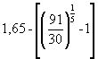 = 1,40
g
t = 1,40 ´ 1,15 = 1,611,615 ´ 649 ´ 10-4 = 0,70 £ 1
Þ
Safety (first case)Table 7 Calculation of total damage in Example of calculation procedure
|
Period |
Tn (years) |
Train (type) |
Speed km/h |
Trains/ day |
l Tj |
( lTj)k |
S NjN (lTjn)k |
1 - j |
[(1+j)/fuci]k |
|
|
(1) 1902 - 1908 |
7 |
3.1 3.2 |
60 40 |
20 20 |
0,466 0,529 |
0,021 0,041 |
0,42 0,82 |
1,513 1,337 |
0,97 0,52 |
2,85 2,98 |
|
(2) 1009 - 1923 |
15 |
4.1 4.2 4.3 |
60 80 40 |
20 15 20 |
0,477 0,580 0,484 |
0,024 0,065 0,026 |
0,493 0,984 0,531 |
1,513 1,69 1,337 |
0,97 1,69 0,52 |
7,17 24,94 4,14 |
|
(3) 1924 - 1938 |
15 |
4.3 5.1 5.2 5.3 |
40 80 100 40 |
20 20 15 15 |
0,484 0,657 0,667 0,748 |
0,026 0,122 0,131 0,234 |
0,531 2,44 1,96 3,51 |
1,337 1,69 1,9 1,337 |
0,52 1,69 3,05 0,52 |
4,14 61,95 89,37 27,37 |
|
(4) 1939 - 1953 |
15 |
5.3 6.1 6.2 6.3 |
40 80 100 40 |
20 15 15 15 |
0,748 0,672 0,699 0,814 |
0,234 0,137 0,166 0,357 |
468 2,05 2,49 5,35 |
1,337 1,69 1,9 1,337 |
0,52 1,69 3,05 0,52 |
36,50 51,96 113,9 41,73 |
|
(5) 1954 - 1968 |
15 |
7.1 7.2 7.3 7.4 8.2 8.4 |
80 80 100 40 80 40 |
15 10 10 20 15 15 |
0,252 0,658 0,66 0,883 0,515 0,805 |
0,001 0,123 0,125 0,536 0,036 0,338 |
0,015 1,23 1,25 10,7 0,54 5,07 |
1,69 1,69 1,9 1,337 1,69 1,337 |
1,69 1,69 3,05 0,52 1,69 0,52 |
0,38 31,18 57,18 5,56 0,38 15,75 |
|
(6) 1969 - 1983 |
15 |
8.1 8.2 8.3 8.4 |
80 80 100 60 |
20 25 25 20 |
0,252 0,515 0,67 0,805 |
0,001 0,036 0,135 0,338 |
0,02 0,9 3,37 6,76 |
1,59 1,59 1,64 1,44 |
1,25 1,25 1,46 0,76 |
5,62 16,87 63,15 76,95 |
|
|
|
|
|
|
|
|
|
|
|
S = 747 |
