ESDEP WG 6
APPLIED STABILITY
To establish general criteria for elastic stability and neutral equilibrium as preparation for the use of energy methods in the assessment of critical loads in Lecture 6.4.
Lecture 6.1: Concepts of Stable and Unstable Elastic Equilibrium
Lecture 6.3: Elastic Instability Modes
Lecture 6.4: General Methods for Assessing Critical Loads
Lecture 6.5: Iterative Methods for Solving Stability Problems
Structural design requires that the equilibrium configuration for the structure, under the prescribed loading, is determined and that this can be confirmed as stable; the analysis of stability problems is generally done using energy criteria. In this lecture, the Principle of Virtual Work and the Principle of Stationary Total Potential Energy are presented. The general energy criteria for elastic stability derived from these are established and the determination of critical loading corresponding to neutral equilibrium is explained. Only fully conservative systems are considered. The established criteria are illustrated by two basic examples of rod and spring systems.
The design of structures requires determination of the internal equilibrium forces (moments, shears, etc.) in the structure, under given loadings, and confirmation that the structure is stable under these conditions. It is of fundamental importance to be sure that a structure, slightly disturbed from an equilibrium position by forces, shocks, vibrations, imperfections, residual stresses, etc., will tend to return to it when the disturbance is removed; this required characteristic of elastic stability has become more and more critical nowadays with the increasing use of high strength steels resulting in lighter and slenderer structures.
The theory of elastic stability (buckling) gives methods for determining the following:
Most of these methods are derived from general energy criteria which come from energy principles of mechanics. Therefore, the purpose of this lecture is to briefly present to the student and the practising engineer the principles of mechanics required to understand the general criteria of elastic stability, thereby giving a better understanding of the methods used in buckling investigations, especially the energy methods discussed in Lecture 6.4.
The scope of this lecture is restricted to:
It should be noted that only the static aspect of stability is considered.
In this lecture, changes in the configuration of a system from an initial configuration are considered; any change in the configuration is to be regarded as a displacement. A configuration can be specified by means of a finite number of independent real variables, called generalised coordinates, denoted here as q1, q2, ... qn or more generally qi. A single-span beam may, of course, possess an infinite set of generalised coordinates, such as the coefficients qi of a Fourier series, that represent its deflection:
y = ![]() qi sin ipx/L
qi sin ipx/L
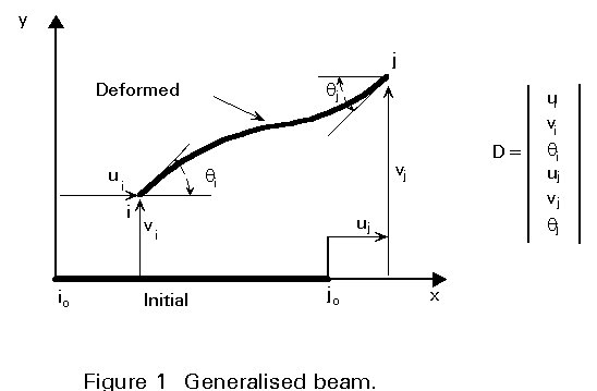
This series, however, can be approximated by a finite number of terms with a finite number of generalised coordinates which denote the degrees of freedom of the system. Considering the beam in Figure 1, the generalised coordinates could be the degrees of freedom of the nodes i and j at the ends of the beam: two translations u and v and one rotation q per node (all in plane). It is assumed here that the entire elastic deformed shape of the beam can be defined by using, for example, interpolation functions. The displacement vector of the beam can be denoted D = (ui, vi, qi, uj, vj, qj).
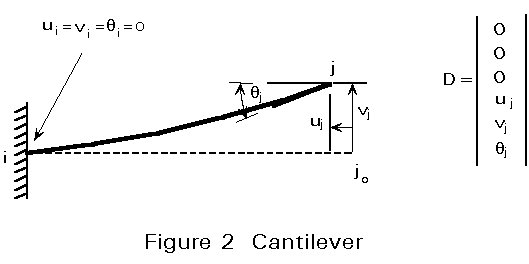
At supports, boundary conditions impose restrictions on the generalised coordinates. In Figure 2, for example, the boundary conditions are such that the displacement vector vanishes at the clamped end of the cantilever beam, such that the restrictions ui = vi = qi = 0, are imposed.
A structural system is generally subjected to internal and external forces; internal forces are generally tractive forces, i.e. forces due to stresses, on the faces of infinitesimal cuboids in the material. External forces can act on the volume (for example gravity) and/or the surface (such as contact forces or couples) of the elements of the structural system.
During a change in the configuration of the system, the Law of Conservation of Energy may be expressed by:
Wext + Q = DT + DU (1)
where: Wext is the work performed on the system by external forces
Q is the heat that flows into the system
DT is the increase of kinetic energy
DU is the increase of internal energy
U is also commonly called strain energy.
On the other hand, the Law of Kinetic Energy is expressed by:
W = Wext + Wint = DT (2)
where: Wint is the work performed by internal forces
W is the total work performed on the system by all forces
Equations (1) and (2) yield:
Wint = Q - DU (3)
Because only adiabatic processes are considered here, Q = 0 and Equation(3) yields:
Wint = - DU (4)
Note: DU exists only for deformable systems; for a rigid system:
DU = 0 so Wint = 0 (5)
Because only static aspects are considered here, no variation in the kinetic energy is supposed to occur during the displacement (very slow speed):
DT = 0 (6)
and Equations (1), (2) and (5) yield:
Wext = DU (7)
Wext + Wint = 0 (8)
The analysis of stability problems generally uses the Principle of Virtual Work which will be discussed in this Section. First, the problem is to find the true equilibrium configuration for the system, if it exists, and then to test its stability.
A given system can take up any number of displaced configurations within the limitations of the boundary conditions but only one of these is the true one, which corresponds to equilibrium between the actual applied loads and the induced reactions.
Suppose that the system is in a configuration specified by the generalised coordinates q1, q2, ... qn, which is to be tested for equilibrium.
Suppose the system experiences some arbitrarily small displacements from this configuration, merely required to satisfy the boundary conditions, but with the actual loads acting at their fixed prescribed values. The small displacements considered here are not necessarily realised; they are imagined to occur purely for comparison purposes, and so they are called virtual displacements; these virtual displacements are independent of the loading and are denoted here dqi. Consequently, all work or energy calculations carried out on the system will lead to virtual work or energy.
For a rigid system, Equations (5) and (8) yield:
dWext = 0 (9)
where dWext is the virtual work of external forces going through the virtual displacements; the Principle of Virtual Work may be expressed as follows:
"A rigid system is in its equilibrium configuration if the virtual work of all the external forces acting on it is zero in any virtual displacement which satisfies the boundary conditions."
For a deformable system, Equation (7) yields:
dWext = dU (10)
where dU is the variation of strain energy in the virtual displacement, and the Principle of Virtual Work may be expressed as follows:
"A deformable system is in its equilibrium configuration if the virtual work of all the external forces acting on it is equal to the variation of strain energy in any virtual displacement which satisfies the boundary conditions."
This is the form of the principle frequently quoted in structural analysis; it is equivalent to the condition, using Equation (8):
dW = dWint + dWext = 0 (11)
True Equilibrium Configuration
For a system with a finite number of generalised coordinates (q1, q2, ...qn), the virtual work dW corresponding to a virtual displacement from a configuration (q1, q2, ...qn) to a neighbouring configuration (q1 + dq1, ...qn + dqn) may be represented by a linear form in the variations of the coordinates, that is:
dW = Q1.dq1 + Q2.dq2 + ... = ![]() Qi dqi
i=1,2,...,n (12)
Qi dqi
i=1,2,...,n (12)
where Q1, Q2, ...Qn are certain functions of generalised coordinates qi, and of internal (for deformable systems) and external forces.
By analogy to the work performed by a force, the functions Q1, Q2, ... Qn are called components of generalised forces. The terms Qi do not necessarily have the dimension of force and they frequently do not all have the same dimension; their dimensions are determined by the fact that Qi dqi has the dimension of work. Equations (11) and (12) yield:
![]() Qi dqi = 0
i=1,2,...,n (13)
Qi dqi = 0
i=1,2,...,n (13)
As dqi are arbitrary, independent of variations in qi, Equation (13) implies that:
Qi = 0 i=1,2,...,n (14)
Solution of these n simultaneous equations of equilibrium yields the values of the q's corresponding to the true equilibrium configuration.
The internal and external forces are both conservative (fully conversative system). The internal forces derive from the single scalar function of the generalised coordinates U(q1, q2, ...qn) whose value U is the strain energy which is expressed by Equation (4). Similarly, the external forces derive from the function W(q1, q2, ...qn) whose value W is the potential energy of these forces. It yields the result that all forces derive from the single scalar function V (q1, q2, ...qn) which is called the total potential function and whose value is the total potential energy of the system. This total potential energy may be expressed as:
V = U + W (15)
The total amount of potential energy is generally indeterminate. Only changes of potential energy are measurable and can be investigated.
Because the system is assumed to be fully conservative,
dW = - dV (16)
where dV is the variation of total potential energy in the virtual displacement, and (11) and (16) yield:
dV = 0 (17)
Equation (17) is an analytical statement of the Principle of Stationary Total Potential Energy which states:
"Of all the geometrically possible configurations which a system can take up, the one corresponding to equilibrium between the applied loads and the induced reactions, is that for which the total potential energy is stationary."
True Equilibrium Configuration
Since V = V(q1, q2, ...qn), dV may be expressed by:
dV = ![]() (18)
(18)
Here, the values of dqi are arbitrary and independent so that if dV = 0, then:
![]() (19)
(19)
Thus the principle provides n equations of equilibrium expressed in terms of the applied loads and the generalised coordinates qi from which the values of qi, defining the equilibrium configuration, can be found.
It should be noted that Equations (12), (16), (18) and (19), and the fact that the values of dqi are arbitrary and independent, give:
![]() = - Qi = 0 i = 1,2,...n (20)
= - Qi = 0 i = 1,2,...n (20)
In summary, it should be noted that for fully conservative systems, the Principle of Virtual Work becomes the Principle of Stationary Total Potential Energy. The principle is exact and very powerful and can be used to develop approximate methods for solving stability problems in structural design.
A system is said to be in a stable state of equilibrium if, after the removal of some slight disturbance, it tends to return to its original equilibrium configuration. If the slight disturbance results in the system departing from the equilibrium configuration, then it is unstable. One can conceive of an intermediate situation in which the slightly disturbed configuration is maintained when the disturbance is removed. This situation is a state of neutral equilibrium. It has been illustrated in Lecture 6.1 with the well-known example of ball in a saucer. Evidently, the slight displacements contemplated must be in accordance with the boundary conditions so that they correspond to slight changes in the generalised coordinates of the system; a discussion of the stability of equilibrium can thus be based on virtual displacements.
The Principle of Virtual Work shows that the potential energy is stationary at equilibrium; it has also been shown, in Lecture 6.1, that it is at a relative minimum when the equilibrium is stable; the condition for stability may therefore be stated in the form:
"The existence of a relative minimum of the total potential energy in the equilibrium configuration constitutes both a necessary and a sufficient condition for the stability of this configuration."
If DV denotes the increment of total potential energy consequent upon a virtual displacement from the equilibrium configuration, then:
DV > 0 for stable equilibrium
DV = 0 for neutral equilibrium (21)
DV < 0 for unstable equilibrium
It can be seen that, because the potential energy is stationary at equilibrium (dV = 0), a discussion of stability involves a discussion of the higher order terms appearing in the increment of potential energy DV.
The function V(q1,q2,...qn) and its partial derivatives to the third order with respect to qi are postulated to be continuous functions of qi; then by Taylor's series in the vicinity of the initial equilibrium configuration, the increment DV of V corresponding to virtual variations dqi of qi, is:
D
V =or DV = dV + ![]() d2V + 0(d3)
(23)
d2V + 0(d3)
(23)
with d2V = ![]() dqi dqj
i,j = 1,2,...,n (24)
dqi dqj
i,j = 1,2,...,n (24)
0(d3) is a third order small quantity.
The Principle of Virtual Work means that a necessary condition for equilibrium is that dV vanishes for all dqi, that is:
dV = 0 or ¶V/¶qi = 0 i = 1,2,...,n (25)
The sign of DV is therefore governed by the sign of d2V, so taking into account Equation (21), the condition for stability becomes:
d2V > 0 (26)
If:
aij = ![]() (27)
(27)
then d2V = ![]() aij
dqi dqj
i,j = 1,2,...,n
(28)
aij
dqi dqj
i,j = 1,2,...,n
(28)
Introducing the matrix [a] of the coefficients aij, Equation (28) can be written as:
d2V = {dq}t [a] {dq} (29)
The condition for stability (Equation (26)) requires that:
[a] = a positive definite matrix
that is to say that all the principle minors of [a] must be positive.
The coefficients aij are functions of the applied loads and the properties of the system so that positive definiteness of [a] imposes the condition which the loads must satisfy in order that the configuration be stable.
The existence of a relative minimum for the total potential energy when a configuration is stable, and considering the neutral equilibrium as a limit of the stability, the condition for neutral equilibrium may be expressed by:
d2V = 0 = minimum (30)
Considering Equation (29) in the case of the non-trivial configuration {dq} 0, the state of neutral equilibrium is obtained when the matrix [a] is singular.
The coefficients aij of [a] are functions of the geometrical and mechanical characteristics of the system, and also of the applied loads.
It is of practical importance therefore to determine the critical values of loads leading to a neutral equilibrium for the system under which a change in the stability state of the equilibrium configuration occurs.
Introducing a common load multiplier a for all loading components and defining a reference loading system S1 (corresponding to a = 1), loads at any time of a proportional loading history are equal to:
S = a S1 (31)
Only the load multiplier a is unknown and the condition for neutral equilibrium requires the solution of the eigenvalue problem:
det [a(a)] = 0 (32)
Solving Equation (32) leads to a set of solutions a, denoted acr, whose number is equal to the number of generalised coordinates of the system. The eigenvectors represent the deformed configuration associated with each solution a. Most of these mathematical solutions do not correspond to actual behaviour of the structural system; generally, the designer is only interested in the values of loads above which the system, stable when unloaded, becomes unstable. These loads are normally obtained with the smallest positive value a°cr of acr and so, the critical loads are determined by:
Scr = a°cr S1 (33)
Example 1
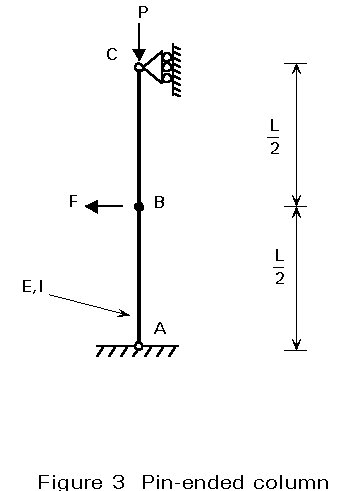
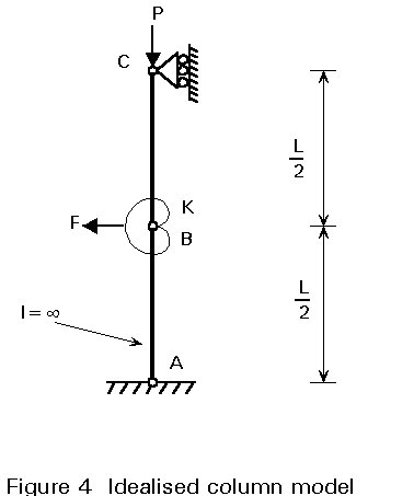
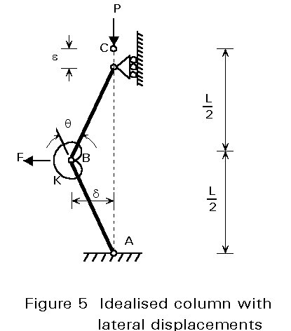
It is interesting to illustrate the stability criterion with the basic example of a pin-ended compression element shown in Figure 3; however, in order to perform very simple strain energy calculations, it is assumed that the whole flexibility of the element is concentrated in a single rotational elastic spring at mid-span, as shown in Figure 4. The two rods, each of length L/2, are rigid so that their strain energy is zero. The value K of the spring, constant at B, will be discussed later. Sideways movement of the pins A and C are fully restrained. The load P acts vertically downwards at C, and the external force F, present from the beginning of loading, acts horizontally leftwards at B.
Because of the boundary conditions, the system has only one degree of freedom. Let us choose the lateral displacement at B as the generalised coordinate denoted d, see Figure 5. (Another possibility would have been to choose the rotation of the lower or upper rod). Before studying the stability of this system, let us determine its equilibrium configuration under the loads P and F. The displacements will be assumed sufficiently small so that trigonometric functions will be reduced to the first term of series development.
The strain energy of the system in its deformed shape is that of the spring only, that is:
U = UO + ![]() Kq2
(34)
Kq2
(34)
where UO is the potential energy of the system in its initial configuration
q is the rotation in the spring (see Figure 5).
It is easy to demonstrate that q = 4d/L and this yields:
U = UO + 8 Kd2/L2 (35)
The potential energy of external loads is:
W = WO - Pe - Fd (36)
where WO is the potential energy of external loads when the system is in its initial configuration
e is the induced vertical displacement at C (see Figure 5)
It can be demonstrated that, for small displacements, e = 2d2/L and this yields:
W = WO - 2 Pd2/L - Fd (37)
The total potential energy is:
V = U + W = VO + 8 Kd2/L2 - 2 Pd2/L - Fd (38)
where VO is the initial potential energy of the system.
According to Equation (19), the equilibrium configuration is given by the solution of:
![]() = (16K - 4PL) d/L2 - F = 0
(39)
= (16K - 4PL) d/L2 - F = 0
(39)
This yields:
d = FL2 / (16K - 4PL) (40)
The condition for stability, from Equation (26), may be expressed by:
![]() = (16K - 4PL) / L > 0
(41)
= (16K - 4PL) / L > 0
(41)
The system will be stable if the following condition is fulfilled:
P < 4 K/L (42)
The value of P at the limit is its critical value Pcr at which elastic buckling occurs. It is worth noting that this critical value is independent of the external lateral force F acting on the system. In particular, this critical load is valid for the particular case F = 0, denoting the classical column buckling problem under axial load only.
A value may be given to K so that the flexibility is the same as the continuous element of Figure 3. It is defined, therefore, as the value that gives the same lateral displacement d at B due to F as the continuous element assuming P is zero.
For the continuous element, simple beam theory gives:
d = FL3 / (48 EI) (43)
where I is the second moment of area of the element section.
E is Young's modulus.
For the rod and spring system, expressing the moment at B with q = 4d/L, gives:
d = FL2 / (16 K) (44)
Equations (43) and (44) yield the equivalent spring constant: K = 3 EI/L, and the critical value of P is equal to:
Pcr = 12 EI/L2 (45)
This value is to be compared to the well-known exact value p2 EI/L2; the accuracy of the result depends, in fact, on the assumptions adopted for the determination of the equivalent spring constant K.
Example 2
Consider now the rod and spring system shown in Figure 6. The two rods AB and BC, each of length L, are rigid (no strain energy) and are pinned and linked together at B. Sideways movement of the pins B and C is restrained by linearly elastic springs, effective in both tension and compression, of stiffness K1 and K2 respectively. The load P acts vertically downwards at C, and the external forces F1 and F2 act horizontally leftwards at B and C respectively.
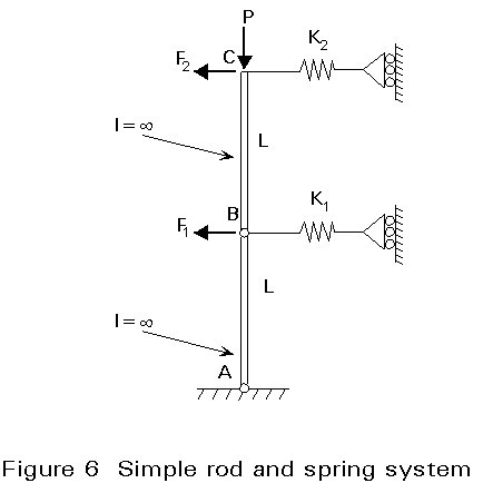
Taking the boundary conditions into account, the system has two degrees of freedom. The rotations q1 and q2 of the two rods are chosen as the generalised coordinates (see Figure 7). The equilibrium configuration of the system is determined first and, secondly, its stability is discussed.

The strain energy of the system is that of the springs only. The strain energy of each spring is equal to Kd2/2 where d is the sideways displacement in the relevant spring and K its stiffness (or spring constant). Consequently, the strain energy in a configuration (q1,q2) is:
U = UO + K1L2q12 /2 + K2L2(q1 + q2)2 /2 (46)
The potential energy of external loads is:
W = WO - PL(q12 + q22) /2 - F1 L q1 - F2 L (q1 + q2) (47)
The potential energy is:
V = U + W (48)
The required derivatives are:
 (49)
(49)
Equilibrium configuration
The condition of stationary potential energy, Equation (19), provides the following set of equations:
{ q1 (K1L2 + K2L2 - PL) + q2K2L2 = (F1 + F2) L (50)
{ q1 K2L2 + q2 (K2L2 - PL) = F2L
The equilibrium configuration (q1, q2) may easily be obtained by solving this set of equations. At this stage, the existence of a solution only requires the determinant to be definite, that is to say:
Determinant = (K2L2 - PL) K1L2 + PL (PL - 2K2L2) 0 (51)
Stability
The condition for stability of an equilibrium configuration is expressed by Equation (26) and the matrix [a], the coefficients of which are given in Equation (27), and is determined as follows:
[a] =  =
=  (52)
(52)
The conditions for stability requires the matrix [a] to be positive and definite, that is to say that the following conditions are satisfied:
(K2L2 - PL) K1L2 + PL (PL - 2K2L2) > 0 (53)
K2L2 - PL > 0 (54)
It should be noted that the first condition incorporates condition (51) for existence of an equilibrium configuration; this results from the fact that V is a quadratic in q's.
It is easy to demonstrate that the more restrictive condition, from Equations (53) and (54), leads to the following stability requirement for the vertical load P:
P < 0,5 L (K1 + 2K2 - (K12 + 4K22 )1/2) (55)
or P > 0,5 L (K1 + 2K2 + (K12 + 4K22 )1/2)
Figures 8 - 10 illustrate results for the case: L = 400, K1 = 20, K2 = 30, and F1 = F2 = 40 (units: kN cm)
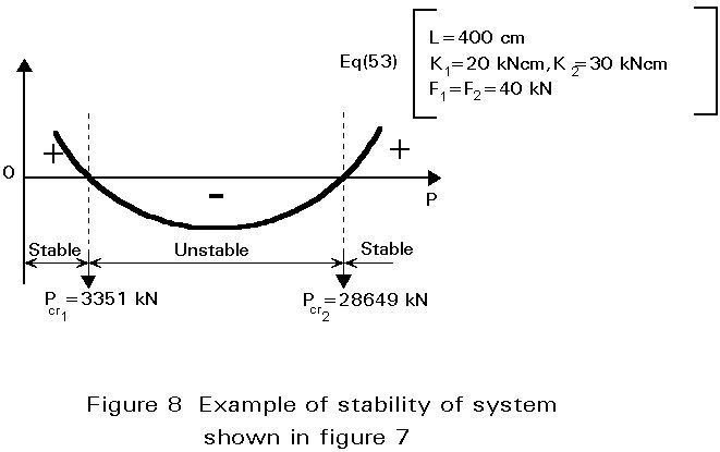

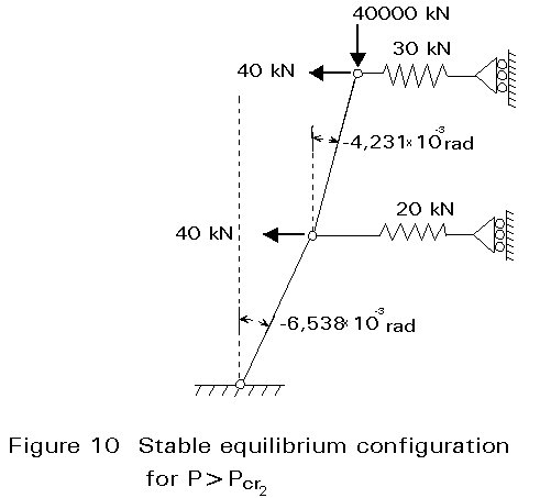
As in Example 1, it is worth noting that the critical values Pcr1 and Pcr2, which bound the unstable domain, are independent of the external lateral forces F1 and F2 acting on the system, and are therefore also valid for the particular case F1 = F2 = 0.