Previous | Next | Contents

Lecture 17.2: Introduction to Seismic

Design - Seismic Hazard and Seismic

Risk

OBJECTIVE/SCOPE

To give an introduction to seismicity, seismic hazard, seismic risk, and seismic measures.

PREREQUISITES

None.

RELATED LECTURES

None.

SUMMARY

The lecture introduces seismicity, explaining the origins of earthquakes and summarises their characteristics in both general and engineering terms. The need for probabilistic assessments is demonstrated and the concept of response spectra is introduced. The basic approaches for design against earthquakes and Eurocode 8[1] are presented.

1. INTRODUCTION

Among the natural phenomena that have worried human kind, earthquakes are without doubt the most distressing one. The fact that, so far, the occurrence of earthquakes has been unpredictable, makes them especially feared by the common citizen, for he feels there is no way to assure an effective preparedness.

The most feared effects of earthquakes are collapses of constructions, for they not only usually imply human casualties but represent huge losses for individuals as well as for the community. Thus, although other consequences of earthquakes may include landslides, soil liquefaction and tsunamis, it is the aim in this lecture to study seismic motion from the point of view of the natural hazard it poses to construction, and particularly to steel structures.

The fundamental goals of any structural design are safety, serviceability and economy. Achieving these goals for design in seismic regions is especially important and difficult. Uncertainty and unpredictability of when, where and how a seismic event will strike a community increases the overall difficulty. In addition, lack of understanding and ability to estimate the performance of constructed facilities makes it difficult to achieve the above mentioned goals.

The future occurrence of earthquakes can be regarded as a seismic hazard, whose consequences represent what can be defined as seismic risk. The separate study of these two concepts is important. The first represents the action of nature and the second the effects on mankind and man-made structures.

2. THE SEISMIC EVENT

2.1 General

The knowledge and study of past seismic events is an important way of predicting the potential seismic hazard for the different zones of the earth. Earthquakes have been reported as far back as during the Babylonian Empire or in 780 BC in China.

A region which has suffered large earthquakes (Figure 1) is the circum-Pacific belt including New Zealand, the Tonga and New-Hebrides Archipelagos, the Philippines, Taiwan, Japan, the Kurile and Aleutian Isles, Alaska, the western coasts of Canada and the United States, Mexico, all the countries in Central America and the western coast of South America from Colombia to Chile. Other regions of the world that also have been subject to devastating earthquakes in the past are the northern and eastern zones of China, northern India, Iran, the south of the Arabian Peninsula, Turkey, all the southern part of Europe including Greece, Yugoslavia, Italy and Portugal, the north of Africa and some of the Caribbean countries.

Worldwide, the most devastating seismic event which has ever happened is believed to be the 1556, January 23rd earthquake in the Shaanxi Province of China. That earthquake may have caused more than half a million casualties. More recently, two other Chinese provinces, the Ningxia province in 1920 and the Hebei province in 1976, were hit by earthquakes that may have caused several hundreds of thousands of dead.

In Europe, earthquakes are reported as far back as 373 BC in Helice, Greece. Other catastrophic earthquakes in Europe occurred in 365, 1455 and 1626 in Naples, 1531 and 1755 in Portugal, 1693 in Sicily, 1783 in Calabria and 1908 in Messina. Each one of these earthquakes is believed to have caused between 30000 and 60000 deaths. Even if these figures are not totally reliable, they give a dimension of the consequences or the risk that may result from the seismic hazard in some European countries.

These major earthquakes have each caused not only a large number of human casualties due to the collapse of houses and other buildings, but also have caused huge economical losses which in some cases took long periods to recover. The large losses, human and economic, that can be expected from the occurrence of future earthquakes justify special attention being given to the study of earthquake phenomena and the earthquake hazard.

2.2 Origins of Earthquakes

Earthquakes have their origin in the sudden release of accumulated energy in some zones of the earth's crust and the resulting propagation of seismic waves.

Wegener introduced the concept of continental drift to explain the origin of the continents, and why the earth's crust is divided into interacting plates. The zones of the earth where most earthquakes are generated are at the boundaries of the plates. Earthquakes occur in some cases due to subduction movements between two plates, as is the case of the Pacific plate which moves underneath the South American continent, and in other cases due to sliding movements between the two plates, as is the case of San Andreas fault in California. In Southern Europe the boundary between the African and the Euroasiatic plates is responsible for some very large earthquakes, as for example the 1755 earthquake that destroyed most of the city of Lisbon.

Other zones where earthquakes occur are at the faults in the intraplate regions, due to the accumulation of strains caused by the pressures in the plate's boundaries. Most of the Chinese earthquakes are generated in the intraplate region. In Europe a similar region is involved for most of the southern part of the continent but also for some other central and northern areas.

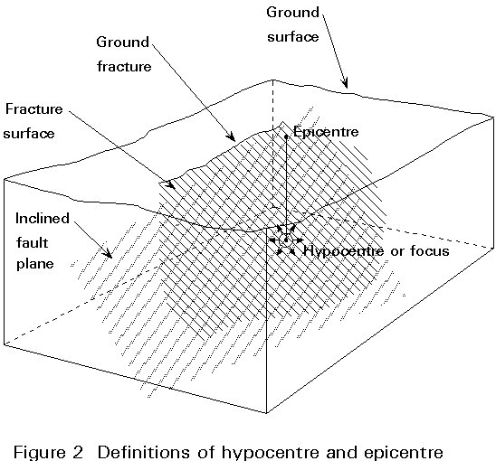
The point or the zone at which the earthquake slip first occurs is commonly designated as the focus or hypocentre. The earthquake focus is usually at a certain depth, known as the focal depth. The intersection of a vertical line through the focus with the ground surface is known as the epicentre (Figure 2). Obviously the most affected zones are the ones closer to the focus, showing that distance to the epicentre (or hypocentre) is a significant factor of seismic hazard.

The sudden release of energy at the focus generates seismic waves that propagate through the rock and soil layers. There are three basic types of seismic waves; P waves, S waves and surface waves which include the Love and Rayleigh waves. The difference of velocity between the P and the S waves allows, by means of the difference in the arrival time, the determination of the hypocentral distance. Typical velocities of P and S waves vary from 100m/sec for S waves in unconsolidated soils (300m/sec for P waves) to 4000m/sec for S waves in igneous rocks (7500m/sec for P waves).

2.3 Earthquake Characteristic

The "size" of the earthquake or what could be seen as a seismic scale is a very important factor for a correct characterization of its potential hazard. Intensity and magnitude are two different means of "measuring" an earthquake which are often confused by the media.

The concept of magnitude which was first introduced by Richter and which still carries his name, represents a measure of the earthquake that is supposed to be independent of the location at which the measurement is obtained. It is related to the amplitude of the seismic waves corrected with respect to distance. It represents a universal measure of the size of the earthquake, independently of its effects. Although there is no maximum value for the magnitude of an earthquake, the two largest magnitudes ever observed correspond to the 1906 earthquake off the coast of Ecuador and the 1933 earthquake off the Sanriku coast in Japan with magnitudes of 8,9. The 1755 earthquake, off the coast of Portugal, is believed to have been the largest earthquake in Europe with a magnitude of 8,6.

The magnitude of an earthquake can be related to other physical measures of earthquakes such as the total released energy, the length of the fault rupture, the fault rupture area and the fault slippage or relative displacement suffered between the two sides of the fault. Several relationships have been proposed by different authors. The ones presented here are merely an indication of the types of relationships. More accurate expressions can probably be presented for different seismic zones. Approximate relationships between magnitude (M), total energy (E in ergs), fault rupture length (L in meters), fault rupture area (A in Km²) and fault slippage displacement (D in meters) are:

Log E = 9,9 + 1,9 M - 0,024 M²

M = 1,61 + 1,182 log L

M = 4,15 + log A

M = 6,75 + 1,197 log D

The relationship between energy and magnitude shows that an earthquake of magnitude 8 releases as much as about 37 times the energy released by a magnitude 7 earthquake. The same observation can be made for the relationships between magnitude and measures of the fault, showing that an increase of one degree in the Richter scale corresponds to a considerable increase in terms of seismic hazard.

A different way of measuring an earthquake, has been adopted, based on a scale initially proposed by Mercalli and later modified, known as the Modified Mercalli Intensity (MMI). According to this scale (Table 1), which varies between I and XII, the intensity of an earthquake is dependent on the observed effects on landscape, structures and people at a given site. Thus, the intensity is variable from place to place and relies on a subjective appreciation of the earthquake consequences. An approximate correspondence between MMI and ground acceleration, a parameter which will be further discussed, is presented in Table 1.

1. At intensity I there may be effects from very large earthquakes at considerable distance in the form of long-period motion. These effects include disturbed birds and animals, swaying of hanging objects, and slow swinging of doors, although people will not feel the shaking and will not recognize the effects as being caused by an earthquake.
2. Each earthquake effect is listed in the table at the level of intensity at which it appears frequently. It may be found less frequently or less strongly at the preceding (lower) level and more frequently and more strongly at higher levels.
3. The quality of masonry or brick construction was categorized by Richter (1956) as follows:

Figure 3 represents a map of the maximum observed intensities in Europe, which is based on the recollection of the effects of past earthquakes, and thus can already be looked at as a measure of seismic risk.

The duration of ground motion is another parameter of great interest when assessing the seismic hazard for a given seismic environment. Although there is no single definition for the duration of an earthquake, all the most commonly used definitions agree as a rule that the duration of an earthquake at a given site increases with the magnitude, epicentral distance, and the depth of the soil above bed-rock. The duration of an earthquake is a very important parameter especially when assessing the non-linear response of structures. The accumulation of structural damage, which is related to the non-linear behaviour of the structure and may lead to structural failure, can be highly affected by the total time a structure is subjected to strong ground motion. An earthquake with a given magnitude may represent a smaller hazard than an earthquake with a smaller magnitude but larger duration or even than a series of smaller magnitude earthquakes.

All the possible measures of an earthquake that have been presented so far, are of limited interest from the engineering point of view. The relationships that have been established between the different parameters are not deterministic and involve a great amount of uncertainty and variability. On the other hand, they relate more to the physical aspects of the seismic source and, except for the Mercalli Intensity which is determined based on subjective judgement, do not take into account the site characteristics and the hypocentral or epicentral distance.

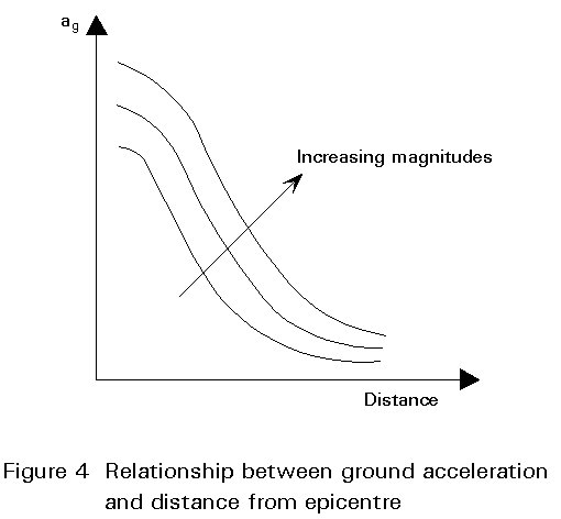
The need for an engineering characterization of the seismic motion, justifies the use of alternative parameters, such as the maximum ground acceleration or peak ground acceleration (a_g) observed during the ground motion at a given site. The maximum acceleration has been observed to be statistically dependent on the magnitude of the earthquake. Hence it is dependent on the severity of the seismic source, and is also highly dependent on the distance to the epicentre and on the soil characteristics and other local site conditions. Figure 4 shows the type of relationship that exists between a_g and distance for different earthquake magnitudes.

Approximate relationships exist between the Richter Magnitude, the Modified Mercalli Intensity and a_g observed in the epicentral zone. However these relationships are very dependent on several other parameters such as the local soil conditions and even on the type of seismic source.

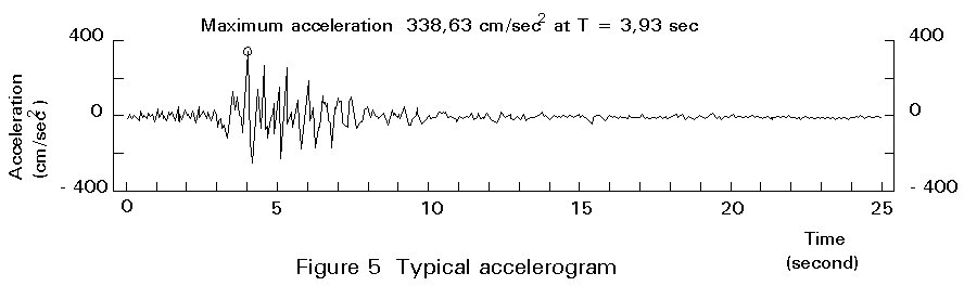
Instruments are available that measure the movements of the ground due to earthquakes. Some instruments measure the ground displacements and are called seismographs. To measure the ground accelerations, other type of device exist, called accelerographs. The accelerographs register the accelerations of the soil and the record obtained is called an accelerogram. A typical accelerogram is represented in Figure 5, showing the peak ground acceleration (a_g).

Knowing, for a given earthquake and site, the accelerations in three orthogonal directions, it is possible to evaluate the response of a structure when subjected to that specific earthquake.

But for a given site, there may be more than one potential seismic source and from a given source earthquakes with different magnitudes, durations and peak ground accelerations may occur. In addition, even for the same earthquake, accelerograms obtained in different locations may vary substantially, depending on the local site conditions. The geometry and properties of the soil have been shown in past earthquakes to have a large influence on the characteristics of the accelerogams obtained. Thus, the accelerograms obtained from past earthquakes have to be used with special care. They may not correctly represent the ground accelerations of future events.

The knowledge of the seismic ground motion is an essential aspect of the characterization of the seismic hazard. Access to accelerograms from different earthquakes, in different seismic environments, for several magnitudes and epicentral distances, in different soil conditions gives a unique basis for characterizing the ground motion and determining its most influential parameter. Arrays of strong ground motion accelerographs have been used in the last decade allowing a more reliable estimate of the earthquake motion. Thus a probabilistic assessment of the earthquake input is obtained for use in engineering applications.

Among the aspects that are investigated with arrays of ground motion accelerographs are the influence of the type of seismic action, hypocentral distance, wave propagation path, orientation of the site with respect to the fault line, local soil conditions and local topography.

During the lifetime of a structure there is a certain probability that it may be subjected to one or more earthquakes. The probability depends on the seismic environment and on the period for which the structure is to function. The probability that an earthquake with a large magnitude, and consequently with large a_g values, occurs during the lifetime of a structure, is smaller than the probability of occurrence of smaller earthquakes. The number of earthquakes (N) having a magnitude (M) or greater per year, can be estimated by means of recurrence formulae of the type.

log N = a - b M

where a and b are parameters depending on local conditions.

For each seismic zone, and based on past seismic events, recurrence formulae can be obtained, giving the annual probability of occurrence of earthquakes with a certain magnitude, or the return period of occurrence of an earthquake with a given magnitude. As the magnitude can be related with a_g, these types of relationship give the return period of occurrence of a certain level of ground acceleration. According to the time period to be adopted, which depends on the level of risk to be accepted, the corresponding a_g value can be determined. This a_g value, is the peak ground acceleration that will be exceeded with a given probability, necessarily very small, and thus assuming a certain level of seismic risk.

Differences between past and future ground accelerations will exist not only in terms of the maximum observed values (a_g) but also in terms of the frequency content. Thus, another aspect that has to be examined in any study of seismic hazard, is the frequency content of the earthquake records. The fourier transform, the spectral density function or power spectrum and the response spectrum are different ways to characterize an accelerogram in the frequency domain. It should be noted that Eurocode 8 recommendations allow the use of accelerograms, power spectra or response spectra to define the seismic motion for structural analysis purposes. The last approach will be discussed here because it is the simplest approach of those available which have direct application to structural analysis.

2.4 Response Spectrum

The response spectrum of a given earthquake record is the representation of some maximum response quantity of a damped, linear, single degree of freedom system as a function of the natural frequency of that system.

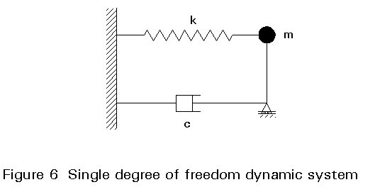
For example, for the system shown in Figure 6, with mass m, stiffness k, (velocity dependent) damping c, ground displacement d_g, and displacement of the mass relative to the ground d_r, the equation of motion can be written in the form

m (d_g'' + d_r'') + cd_r'' + kd_r = 0

or

md_r'' + cd_r' + kd_r = - md_g''

This equation of relative displacement is the same as that for a mass with fixed base subjected to a horizontal force -md_g''. Introduction of the natural frequency of the undamped system w = , the natural period of the undamped system T = 2p/w, and the damping ratio z = c/2mw, gives

d_r'' + 2z wd_r' + w² d_r = -d_g''

with the solution

d_r = -exp (-pw,t)/w_D d_g''(t) exp [z w_D (t - t)] sin w_D (t - t) dt ,

d_i = exp (-z w_D t)/w_D d_g (t) exp [z w_D (t - t)] sin w_D (t - t) dt ,

where

w_D =  Ö(1 - z²) is the natural frequency of the damped system.

z =1 corresponds to the critical damping c_cr = 2.

For a given accelerogram, i.e. given d_g'', the maximum of d_r, for a given value of z, can be determined for each w_D. Usually the value z = 0,05 is used as a reference value and a correction factor h for damping ratios different from 5% is introduced.

A typical acceleration response spectrum for three damping ratio values is shown in Figure 7.

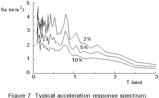
The two parameters that most influence the shape of the response spectrum, or its frequency content, are the type of earthquake and the local soil conditions. The influence of these two parameters on the shape of the spectrum arises from the phenomenon of resonance. In reality the fact that a certain earthquake has a predominance of energy centred in a given frequency range will cause the response spectrum to have larger amplitudes in that same frequency range. Two aspects that may lead to different spectra are the distance of the site to the seismic source and the characteristics of the local soil. Large hypocentral distances tend to diminish the high frequency components of the local ground motion. Soft soils also tend to amplify the low frequency components of the ground motion, whereas for hard soils the high frequency components are amplified.

In the past, it has been observed that similar structures subjected to the same earthquakes show a quite different seismic behaviour because of the local soil conditions. In the 1967 Caracas, Venezuela earthquake, it was observed that damage to buildings was not uniform throughout the city. Tall buildings with foundations on soft thick soil layers showed much more damage than the same type of building with foundations on stiffer soils. The opposite was observed for low-rise buildings; they showed more damage for foundations on the stiffer soils. This observation showed that the same earthquake motion can be filtered in a different way by two distinct soils. Thus the seismic input into a structure may vary according to the local soil conditions. The interaction between the ground motion and the structural characteristics is thus of great importance in the evaluation of the seismic response of structures and the associated seismic risk.

3. EARTHQUAKE INPUT FOR STRUCTURAL DESIGN

The fact that, for a given earthquake source and site, there have been no observed earthquakes with a magnitude, intensity, or peak ground acceleration larger than certain values, does not mean that larger values will not be observed in future. Thus, the maximum possible or probable values have to be derived using a probabilistic approach. Furthermore, if one derives probabilistic maximum values for earthquakes that may occur during a certain future period of time, the values will differ from the ones relating to a different period of time. The return period of an earthquake with given characteristics, can be defined as the inverse of the annual probability of occurrence of that event. The larger the seismic event, the larger the corresponding return period as shown by the recurrence formulae already presented.

If the earthquake for which the structure has to be designed and its return period are known, and if the period for which the structure is designed is also known, the probability of the structure being subjected to the earthquake during its lifetime can be determined. Evaluating this probability is a matter of assessing a parameter of seismic risk. To evaluate the global seismic risk, one should combine this type of information with the information regarding the single probability of collapse or malfunctioning of the structure if designed according to certain levels and standards of resistance and ductility.

Different earthquakes lead to dissimilar response spectra. Not only different maximum values of the ground acceleration (a_g) lead to different maximum spectrum values, but also different accelerograms will result in dissimilar shapes of spectra even with the same a_g. So, the use of response spectra to characterize a certain potential seismic event, has to take into account the influence of important aspects such as the nature and distance of the seismic source and the characteristics of the soil.

For these reasons, the evaluation of response spectra for design purposes must include a probabilistic study of the seismic occurrences. The study will define the maximum ground acceleration and the shape of the spectra to be considered, for each seismic source and each different kind of soil. This definition is usually obtained by statistical means. The spectra used for design purposes, and the spectra presented in regulations are usually the smoothed graphs of the maximum credible values of the corresponding spectra, for a certain level of risk acceptance, in terms of seismic origin and local soil conditions, obtained for different earthquakes.

The different levels of risk acceptance are also related to the importance of the structure to be designed. The catastrophic consequences arising as a result of collapse or malfunctioning of important buildings and other structures, such as hospitals, fire stations, power plants, schools, dams, main bridges, etc. requires design to a lower level of risk than for normal structures. This lower level is achieved by designing these structures to a larger earthquake return period and consequently to higher values of seismic input. This approach corresponds to designing them to a lower probability of damage and collapse in the event of future earthquakes.

Similarly, different levels of probability of occurrence of earthquakes can also be used for different design philosophies. For regular structures, the choice of an earthquake level with a very low probability of being exceeded is usually associated with a design aimed at avoiding structural collapse, and thus human casualties, even if the structure undergoes major damage and has to be rebuilt. For earthquake levels with higher probability of occurrence, and that may thus occur more often during the lifetime of the structure, the design goal is not to avoid collapse but rather to guarantee that no substantial damage occurs and that the structure maintains its serviceability.

Usually, the response spectra are presented in normalized form, as is the case of the normalized elastic response spectrum of Eurocode 8. It is normalized to the peak ground acceleration (a_g), i.e. it is independent of a_g and so can be used for different values of the maximum expected acceleration for the site. This approach allows for the use of the same spectra for different conditions of severity of the ground motion. In other words, it enables the consideration of earthquakes corresponding to different return periods and thus to different acceptance of seismic risk.

According to Eurocode 8 and other national regulations, the elastic response spectrum to be used for design purposes depends on several parameters such as the seismic zone, the type of seismic action, the local soil conditions and the viscous damping ratio of the structure.

The seismic zone can be characterized by means of the severity of the seismic action. This characterization is accomplished by normalizing the response spectra to a certain level of a_g. Usually, the response spectrum for the vertical motion is defined as a percentage of the response spectrum for the two orthogonal horizontal directions. In Eurocode 8 the suggested percentage is 70%.

The maximum acceleration to be used in each region in Europe is defined according to microzonation studies for each zone, depending on the local seismic hazard parameters. It is the responsibility of the National Authorities.

The normalized elastic response spectrum b_e (T) (Figure 8) is defined by means of four parameters, b_o, T₁ T₂ and k, according to the following expressions:

0 < T < T₁ b_e (T) = 1 + T/T₁ (b_o - 1)

T₁ < T < T₂ b_e (T) = b_o

T₂ < T b_e (T) = (T₂/T)^k b_o

where

T is the natural vibration period of the structure, or the inverse of the natural frequency (Hz)

b_o is the maximum value of the normalised spectral value assumed constant for periods between T₁ and T₂

k is an exponent which influences the shape of the response spectrum for vibration periods larger than T₂.

The values of the transition periods T₁ and T₂, also known as the inverses of the corner frequencies, depend essentially on the magnitude of the earthquake and on the ratios between the maximum ground acceleration, ground velocity and ground displacement.

The basic values presented in Eurocode 8 [1] apply to the ground motion at bedrock or in firm soil conditions. If the soil characteristics differ from the ones considered, other values for the parameters can be chosen in such a way that the shape of the response spectrum is modified accordingly. Eurocode 8 considers three different soil profiles (A, B and C). For each soil profile different parameters (b_o, T₁ T₂ and k) apply. The local response spectrum, b_s (T), can be obtained, correcting the elastic response spectrum by a soil parameter S, which is also dependent on the soil profile.

b_s (T) = S b_e (T)

Although the basic form of the response spectrum is uniform, and is common to the designers in every European Community country, the parameters that define the response spectrum are also the responsibility of each National Authority. The parameters can vary from region to region even in a single country. This variation is due to the fact that each European region has different seismicity.

The b_o value is the maximum spectral amplification. It is dependent on the selected probability of being exceeded for the considered peak ground acceleration, on the damping ratio, on the duration of the ground motion, and on its frequency content. According to Eurocode 8, for a 20 to 30 second earthquake and 5% damping, the value of b_o = 2,5 corresponds to a probability of not being exceeded of between 70 and 80% [1].

The exponent k is dependent on the frequency content and the selected probability of being exceeded. It describes the shape of the response spectrum for the higher periods (lower frequencies).

The use of the elastic response spectrum, simultaneously with linear elastic design, does not take into account the capability of a structure to resist seismic actions beyond the elastic limit. If it can be assumed that the structure will behave linearly for small earthquakes, for larger earthquakes it would be almost impossible and non-economical to design structures based on the assumption of linear behaviour. For larger earthquakes it should be assumed that the structure has a certain capacity to dissipate the energy input by the earthquake by means of non-linear behaviour, even if that implies the existence of structural damage although guaranteeing that collapse is avoided.

Thus, for design purposes, and to avoid the necessity of performing non-linear analysis, the concept of structural behaviour factor (q) is introduced, to correct the results obtained by linear analysis and obtain an estimate of the non-linear response. These behaviour factors, which will be presented in more detail in other lectures, take into account the energy dissipation capacity through ductile behaviour. Thus they are dependent on the materials, type and characteristics of the structural system and the assumed ductility levels. Eurocode 8 defines the q values to be adopted in the case of steel structures according to criteria that will be presented in later lectures.

Based on the q factors, it is possible to define the linear analysis design response spectra that can be used for design purposes by means of linear analysis.

The linear analysis design response spectra is defined in Eurocode 8 as follows:

0 < T < T₁ b(T) = a S [1 + T/T₁ (h b_o/q - 1)]

T₁ < T < T₂ b(T) = a h S b_o/q

T₂ < T b(T) = (T₂/T)^k a h S b_o/q

where

T, b_o, T₁, T₂ and k have the same meaning as above.

a is the ratio of the peak ground acceleration to the acceleration of gravity.

h is a conservative factor for damping ratios different from 5%.

q is the behaviour factor which can depend on T.

The influence of the structural damping ratio is obtained by means of:

h = Ö (5 / z); h > 0,70

where z is the value of viscous damping ratio as a percentage.

According to Eurocode 8, if there is a possibility of two earthquake sources affecting a given site, the use of two different response spectra may be necessary to quantify the seismic input and response [1]. This possibility may arise for sites that may be affected by very large magnitude earthquakes with large epicentral distances and simultaneously by smaller but nearby earthquakes. In that case, although the a_g or b_o values may be quite similar, the shapes of the two corresponding spectra may vary substantially (Figure 9). As a result, some structures may be more affected by one of the earthquakes, whereas other structures may be more affected by the other one.

If a more sophisticated approach is required, and non-linear analysis is to be performed, or if alternative design is to be made, the use of earthquake time-histories, or records of ground acceleration, is necessary. When insufficient previously recorded earthquake accelerograms are available or when they do not belong to the same seismic environment, artificially generated earthquakes may be used. There are several alternative methodologies for generating artificial earthquakes. The only constraint is that the generated histories shall be consistent with the response spectrum corresponding to the case under study. The same applies to the use of power spectra to represent the seismic action.

As a final observation on the characterization of the seismic motion, the effects of the spatial variability of the seismic motion should be considered. The seismic input may be different from support to support. The differences are due to several factors such as the overall dimensions of the structure, the large distances between two supports of the same structure, or the fact that a structure may have different foundation conditions, both in terms of soil or foundation types. In this case a spatial model of the seismic action has to be used, taking into account a model of the wave propagation.

4. FINAL REMARKS

The social consequences of earthquakes, in terms of human casualties and injuries and direct and indirect economic losses justify the need to be prepared for earthquakes. Earthquakes are still difficult to predict and, even if they could become predictable, would pose a threat to buildings and other structures. Thus, being prepared for earthquakes consists mainly in proper structural design procedures for seismic loading. To achieve a correct design procedure and thus diminish the seismic risk, it is necessary in the first place, to have a correct knowledge of the seismic input, or the seismic hazard. Simultaneously with the study of the behaviour of structures when subject to seismic loading it is thus fundamental to study the seismic motion, its origin, and the parameters that most influence the characteristics of the motion.

5. CONCLUDING SUMMARY

• Earthquakes are natural phenomena that have caused tremendous losses of lives and goods worldwide including in some large areas of Europe.
• To design structures that can resist earthquakes requires an understanding of the seismic hazard.
• "Measuring" the earthquake can be achieved by means of different parameters such as magnitude, intensity, peak ground acceleration, power spectrum and response spectrum. Parameters that influence the characteristics of the earthquake motion and its response spectrum are the duration and frequency content of the motion and the local soil conditions.
• The response spectrum approach presented in Eurocode 8 which can be used for structural design takes into account a probabilistic approach of the definition of the seismic motion [1].

6. REFERENCES

[1] Eurocode 8: "Structures in Seismic Regions - design", Commission of the European Communities, Report EUR 12266, 1989.

7. ADDITIONAL READING

1. Clough, R. W. and Penzien, J., Dynamics of Structures,

McGraw-Hill - International Student Edition, 1975.

2. Gere, J. M. and Shah, H. C., Terra Non Firma - Understanding and preparing for earthquakes, Stanford Alumni Association, Stanford, USA, 1984.
3. Catalogue of European earthquakes with intensities higher than 4,

Commission of the European Communities, Report EUR 13406, 1991.

4. Dowrick, D. J., Earthquake Resistant Design, Wiley and Sons, 1987.

Previous | Next | Contents