ESDEP WG 6
APPLIED STABILITY
To explain the energy methods for assessing critical loads for cases where it is not possible to get a closed-form solution to differential equilibrium equations.
Beam theory
Lecture 6.1: Concepts of Stable and Unstable Elastic Equilibrium
Lecture 6.2: General Criteria for Elastic Stability
Lecture 6.3: Elastic Instability Modes
Lecture 6.5: Iterative Methods for Solving Stability Problems
When certain assumptions are made about the nature of the deformation of an elastic system during the change of configuration associated with the buckling mode, the elastic system may be approximated by one involving suitable and adjustable parameters which are determined in order that the neutral equilibrium conditions are fulfilled. Using this concept practical approximate methods can be derived which are very useful to the design engineer; some of the best known of these methods are presented in this lecture, i.e. the Rayleigh coefficient, the Rayleigh-Ritz method, and the Galerkin method. An outline of some numerical methods, such as the Euler finite difference method and the finite element method, is also given.
Critical stability loads may be determined using either of the following methods:
The solution of differential equilibrium equations to satisfy prescribed boundary conditions presents many difficulties and can only be achieved for simple buckling problems for structures with low degrees of freedom; such basic problems are presented and solved, in this way, in Lecture 6.3. This approach, however, will not be considered further in this lecture which instead concentrates on the alternative energy methods mentioned above. It should be noted that powerful iterative methods can also be used to solve stability problems; some of these methods are presented in Lecture 6.5.
When certain assumptions are made about the nature of the deformation of an elastic system during the change of configuration associated with neutral equilibrium (buckling mode), this elastic system may be approximated by one involving suitable and adjustable parameters or generalised coordinates which are to be determined in order that the neutral equilibrium conditions are fulfilled. This idea provides approximate methods which are very useful to the practical engineer; the best known of these methods are presented in this lecture, i.e. the Rayleigh coefficient, the Rayleigh-Ritz method, and the Galerkin method. An outline of some numerical methods, such as the Euler finite difference method and the finite element method, is also given.
If the adjustable parameters mentioned above are judiciously chosen and of adequate number (in the case of an approximation of a continuous system), these approximate methods will give results very close to the exact solution, at the expense of an increased design effort.
The energy methods for the solution of elastic stability problems are based on the principle of existence of a relative minimum of the total potential energy at neutral equilibrium (see Lecture 6.1 and Lecture 6.2).
It is stated that: considering the change DV, of total energy V of a system, from a starting equilibrium configuration to an adjoining configuration defined by an infinitesimally small and kinematically admissible virtual displacement, then the condition of neutral equilibrium is governed by the second variation d2V of the increment DV, that is:
d
2V = 0 = minimum (1)Generally, when considering steel structures, the stability of a structural system under a set of external loads is studied by considering a buckling deformation, f, from a starting configuration, and performing calculations, according to Equation (1), either to check the stability of this starting configuration, or to determine critical values of external loads leading to instability. The deformation f is expressed as a function of one or more independent variables (generally cartesian coordinates); for example, f(x) as the deflection of a beam or f(x,y) as the deflection of a plate. The change of deformation of a system at neutral equilibrium - the buckling deformation or buckling mode - will hereafter be denoted f(X), where X is the coordinate field of the reference system used (one, two or three dimensions). The function f can be continuous if the system is continuous, or can be defined by intervals if the system is discrete.
Solving Equation (1) requires evaluation of the potential function d2V with respect to the function f, inside a domain of integration noted D (length for a beam, area for a plate, for example). Generally d2V involves quadratic and homogeneous quantities with respect to the buckling deformation f(X) and its derivatives, and is a linear function of the external applied loads.
Introducing a common load multiplier, a, for all loading components and defining a reference loading S1 (corresponding to a = 1), the loads at any time of a proportional loading history are equal to:
S = a S1 (2)
Thus, generally, the function d 2V can be evaluated by:
d
2V(f) =where the function F also involves geometrical and material characteristics of the domain.
Solving Equation (3) with respect to f will lead to determining the values of the loads (via the load multiplier a) at neutral equilibrium, i.e. critical values of loads above which the starting configuration becomes unstable.
The method of calculation of critical loads by Rayleigh coefficient is derived directly from Equation (1); the second variation d2V of the total potential energy may be expressed as follows:
d
2V(f) = d2U(f) + d2W (f,S) (4)where: d2U is the second variation of strain energy (a quadratic and homogeneous function of f); it represents the strain energy corresponding to the buckling mode;
d2W is the second variation of potential energy of external loads S (a linear function of S and a quadratic and homogeneous function of f). It represents the opposite to the work of the external loads corresponding to the buckling mode.
At neutral equilibrium, a (see Equation (2)) takes the particular value acr which is the critical load multiplier above which instability occurs. Equations (1), (2) and (4) yield:
d
2V(f) = d2U(f) + acr . d2W (f,S1) = 0 = minimum (5)If the buckling deformation f is known, the critical load multiplier may be obtained from Equation (4); that is:
a
cr = -Considering now an approximation f1 of f (f1 different from f), acr being known. Then, because of the minimum condition:
d
2V(f1) = d2U(f1) + acr . d2W (f1,S1) > 0 (7)Equations (5) and (7) yield:
acr = - ![]() whatever f1 ¹ f (8)
whatever f1 ¹ f (8)
that is acr < min ![]() whatever f1 ¹ f (9)
whatever f1 ¹ f (9)
This defines the Rayleigh Principle which states that the critical load multiplier acr, calculated using Equation (6) with any kinematically admissible displacement different to the true buckling deformation, will give a value of acr greater than the exact value.
Assuming f1 = f + e f2, where f2 is any kinematically admissible displacement and e is a constant, this gives:
a
cr1 = -where 0(e2) is a quantity in e2. This implies that a first order error in the choice of f gives a second order error in the value of acr. If calculations are performed, using Equation (6) with a good approximating function f, simply required to satisfy the boundary conditions, a precise value of acr may be obtained, with an excess error.
The Rayleigh-Ritz method assumes that the exact solution f(X) of the variational problem described by Equation (3) can be approximated by a linear combination of suitably chosen "coordinate functions" f1(X), f2(X), ... fn(X). That is:
fn(X) = q1f1(X) + q2f2(X) + ... + qn fn(X) (11)
where the q's are constants to be determined, and are to be regarded as generalised coordinates (degrees of freedom) of the system.
When f(X) is approximated by fn(X) in this way, the function d2V, which is to be evaluated, becomes a quadratic and homogeneous function of the q's; Equation (3) can, therefore, be written as:
d
2V = {q}t [a] {q} = 0 (12)where {q} is the vector of the q's and [a] is a matrix whose coefficients aij are:
aij = ![]() (13)
(13)
The coefficients aij are functions of the load multiplier a and the properties of the system.
Considering the case of non-trivial configurations, {q} 0, Equation (12) for neutral equilibrium requires [a] to be a singular matrix, that is to say that the determinant of [a] must be zero. This condition provides an equation in a, of degree n, whose smallest positive solution is to be regarded as the critical load multiplier acr.
The functions fi are chosen in advance, depending on the knowledge and assumptions made about the nature of the deformation. They are not unknown and, provided they satisfy the forced (or geometric) boundary conditions for any value of the q's, the choice of "shapes" is arbitrary. It should be noted, however, that the efficiency of the method does depend on a judicious choice for the f's and that it is an advantage to satisfy all the boundary conditions: in practical applications, one will have some idea of the general nature of the true solution f(X) so that the question of using "outrageous" shapes for the f's rarely occurs. If the functions are judiciously chosen, very good accuracy can be attained with relatively few functions. The efficiency of the Rayleigh-Ritz process may be considerably enhanced if, in addition to the forced (or geometric) boundary conditions (concerning translations or rotations at supports, i.e. f and f´), the natural (or mechanical) boundary conditions (concerning curvature, i.e. f² ) are also satisfied.
To get an idea of the accuracy of the results, a more elaborate procedure is used to obtain a sequence of successive approximations; thus, the following may be taken as a first approximation:
f1(X) = q1f1(X) (14)
and as a second approximation:
f2(X) = q1´ f1(X) + q2´ f2(X) (15)
and successive approximations in a similar way.
Comparison of successive solutions then gives some indication of how accurate the current solution is. It is worth noting that the solution fi + 1(X) will always be better, or at least no worse, than the preceding solution fi(X).
In contrast to the Rayleigh-Ritz method which gives a solution after forming the variational problem, the Galerkin method provides approximate solutions to the differential equations directly, and is applicable whether the transformation into a variational problem is possible or not. It therefore seems to have wider scope than the Rayleigh-Ritz technique and is more attractive in practice since there is no need to evaluate the potential function. It can be demonstrated, however, that the two methods are closely related. The Galerkin method proceeds as follows.
Generally, the governing differential equation of a buckling problem can be written as follows:
L[f(X)] = 0 (16)
where f(X) is the buckling deformation and L stands for a linear and homogeneous differential operator.
Suppose that the exact solution f(X) of Equation (16), is expressible in the form of a complete series of functions:
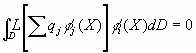
f(X) = ![]() qj fj(X)
(17)
qj fj(X)
(17)
satisfying all the required boundary conditions; the "exactness" of this solution can be expressed by the statement that the left hand side of Equation (16) is orthogonal to every term in the series of Equation (17); that is:
![]() L[f(X)]fj(X) dD = 0
j=1,2,... (18)
L[f(X)]fj(X) dD = 0
j=1,2,... (18)
Suppose the series of Equation (17) is truncated to a finite number of terms, n, then using the above idea, n conditions of orthogonality may be imposed, as follows:
 i=1,2,...n
(19)
i=1,2,...n
(19)
This can be written as follows because L is a linear operator:
![]() L[fj(X)]fi(X) dD = 0
i=1,2,...n
(19´)
L[fj(X)]fi(X) dD = 0
i=1,2,...n
(19´)
This provides an averaging basis for evaluating the n unknown q's such that:
fn(X) = ![]() qj fj(X)
(20)
qj fj(X)
(20)
which constitutes an approximate solution to the differential equation.
The left hand side of Equation (19), which involves properties of the system and external loads via the load multiplier a, is quadratic and homogeneous in q's; this equation can be written in the form of Equation (11) and then treated in the same manner as for the Rayleigh-Ritz method to find the critical loads.
Numerical methods that require the use of a computer may be used to determine the critical loading. An outline of the Euler finite difference method and the Finite Element Method is now given.
Euler Finite Difference Method
In the Rayleigh-Ritz method, it is required that the admissible functions be continuously differentiable throughout the region of integration. The admissible range may be extended by admitting functions having piecewise continuous derivatives. Therefore, the basis of Euler's method of finite differences is to divide the region of integration into a certain number of sub-regions or intervals, assuming linear functions within each one. If fi denotes the value of the function f at the frontier between intervals i and i+1, derivatives of f may be expressed as functions of the f's, and the sum of the second variation of energy over all the intervals is also a function of f's. Here, the f's are to be regarded as the q's in the Rayleigh-Ritz method; Figure 1a illustrates this approach.
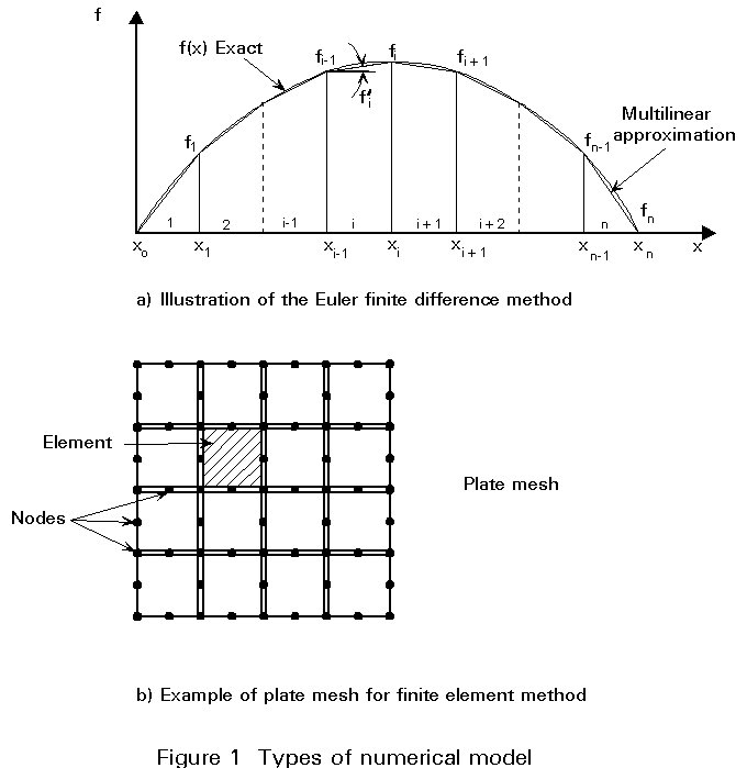
Finite Element Method
This method is used especially for solving stability problems for plate and shell structures. The solution of plate-buckling problems by means of Finite Element theory has been increasing in popularity because it makes use of a matrix formulation suitable for computing. The Finite Element Method has the character of a "piecewise" Rayleigh-Ritz technique; the plate is 'cut' into a number of flat elements joined only at specified nodes, and continuity and equilibrium are established at these nodes. A large number of small elements gives a virtually continuous structure, the behaviour of which is similar to a complete plate. Mixed boundary conditions and varying flexural rigidity can be examined without difficulty. Complete structures may be analysed and post-critical behaviour may also be investigated. An example of a plate mesh is shown in Figure 1b.
Strain energy expressions are needed to perform calculations using the various energy methods. Given below are some useful typical strain energy expressions for structural elements, such as members and plates. These expressions denote the change of strain energy corresponding to the buckling deformation.
Members
Notation
L member length
E Young's modulus
G shear modulus
A cross-section area
Av cross-section shear area
I second moment of area
Iw warping constant
It torsion constant
x abscissa along the member (origin at the beginning of the member)
u(x) axial elongation in member at x }
w(x) lateral deflection in member at x } components of
q
(x) slope due to curvature alone in member at x } bucklingy
(x) shearing angle (dw/dx - q(x)) in member at x } deformationf
(x) torsion angle in member at x }Strain energy
 (21)
(21) (22)
(22)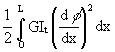 (23)
(23) (24)
(24)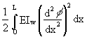 (25)
(25)Thin Plates
Notation
a plate dimension along x axis
b plate dimension along y axis
t plate thickness
x,y cartesian coordinates of any point (origin at a corner of the plate)
w(x,y) deflection
D plate stiffness = Et3/(12(1-u2))
u
Poisson coefficientStrain Energy
Bending:
d
2U =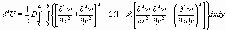 (26)
(26)
Flexural buckling of a compression member is investigated; the critical load is determined using Rayleigh coefficient, Rayleigh-Ritz and Galerkin methods.
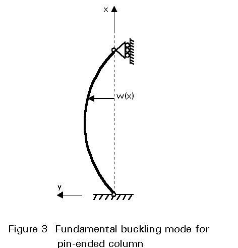
The studied compression member is shown in Figure 2: it is pin-ended and the ends are laterally restrained; L, I and E denote the member length, the second moment of area of the section and Young's modulus respectively; the load P acts vertically downwards; the critical value Pcr of P is to be determined; the buckling deformation of the member is shown in Figure 3.
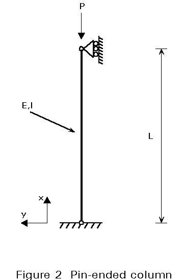
Rayleigh Coefficient Method
The following expression is chosen as an approximation of the buckling deflection w(x):
w(x) = a (x2 - xL) where a = any non zero constant (27)
which satisfies the boundary conditions w = 0 at x = 0 and x = L. The derivatives are:
dw/dx = 2ax d2w/dx2 = 2a (28)
Performing the integration according to Equation (22), the change of strain energy for the buckling deformation is:
d2U = 2a2EIL (29)
The change in the potential energy of P is the opposite of the work done by P for the buckling deformation. The vertical displacement of the point of application of P due to bending deformation is expressed by:
e =  (30)
(30)
and the change of potential energy of external load yields after integration of Equation (30):
d2W = - P e = - P a2L3/6 (31)
The critical load multiplier is obtained by Equation (6), that is:
acr = ![]() (32)
(32)
and, from Equation (2), the critical value Pcr is as follows:
Pcr = 12 ![]() (33)
(33)
This value is to be compared with the exact value obtained from the exact buckling deflection:
w(x) = a sin px/L
that is:
Pcr = p2 ![]() = 9,8696
= 9,8696 ![]() (34)
(34)
This shows that a parabolic buckling deflection is not a very good approximation of the exact buckling mode. If as an approximation the deflection of a simply supported beam under a uniformly distributed load is chosen, that is:
w(a) = a (x4 - 2x3L + xL3) (35)
the above calculations give:
Pcr = 9,88 ![]() (36)
(36)
which is very close to the exact value given in Equation (34).
Rayleigh-Ritz Method
To simplify calculations, the origin of the abscissa is set at mid-length of the member (see Figure 4). A buckling deflection is chosen which is a linear combination of the two following coordinate functions:
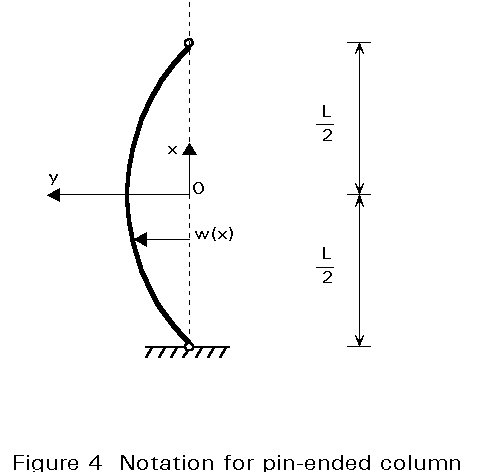
f1(x) = x2 - L2/4 (37)
f2(x) = x4 - L4/16 (38)
which both satisfy the boundary conditions w = 0 at x = -L/2 and x = L/2.
Therefore the expression for the buckling deflection is:
w(x) = a f1(x) + bf2(x) = a (x2 - L2/4) + b(x4 - L4/16) (39)
The derivatives are:
dw/dx = 2ax + 4bx3 d2w/dx2 = 2a + 12bx2 (40)
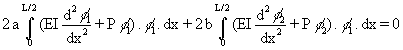
The change in strain energy is expressed by:
d
2U = 2. dx = EI (2 a2L +
 The change in the potential energy of the compression load is expressed by:
d
2W = -2 . dx = - P
 and Equations (4), (41) and (42) give:
d
2V = a2 (2EIL - PL3/6) + b2 (9EIL5/10 - PL7/56) + ab (2EIL3 - PL5/10) (43)The required derivatives are:
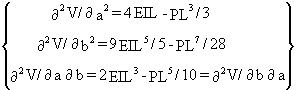 (44)
(44)
and the matrix [a] of Equation (22) is:
[a] = 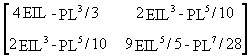 (45)
(45)
Its determinant is given by:
Det [a] = (4EIL - PL3/3) (9EIL5/5 - PL7/28) - (2EIL3 - PL5/10)2 (46)
The smallest positive solution of Det [a] = 0 is:
Pcr = 9,875 ![]() (47)
(47)
which is to be compared to the exact value given in Equation (34). Although the coordinate functions (37) and (38) are individually not really good approximations of the exact buckling mode, their combination (2 degrees of freedom) gives satisfactory results.
Galerkin method
The same approximation of the buckling deformation and co-ordinate sign convention as for the Rayleigh-Ritz method is chosen:
w(x) = af1(x) + bf2(x) (39)
where f1(x) = x2 - L2/4 (37)
f2(x) = x4 - L4/16 (38)
which both satisfy the required boundary conditions which are w = 0 at x = -L/2 and x = L/2 (no imposed condition for the end rotations).
It has been seen in Lecture 6.3 that the differential equation governing flexural buckling of a compression member is:
EI ![]() + Pw = 0 (48)
+ Pw = 0 (48)
The set of equations obtained from Equation (19´) is:
(49)

The required derivatives are:
d2f1/dx2 = 2 d2f2/dx2 = 12x2
After integration, the following set of equations is obtained:
a.[PL5/30 - EIL3/3] + b.[PL7/105 - EIL5/10] = 0 (50)
a.[PL7/105 - EIL5/10] + b.[PL9/360 - EIL7/28] = 0
A non-trivial solution exists if the determinant of Equation (50) is equal to zero; that is:
(PL5/30 - EIL3/3) (PL9/360 - EIL7/28) - (PL7/105 - EIL5/10)2 = 0 (51)
whose smallest solution is:
Pcr = 9,8697 ![]() (52)
(52)
which is nearly equal to the exact value given in Equation (34).