ESDEP WG 6
APPLIED STABILITY
To introduce the main concepts and definitions required for the understanding of stable and unstable elastic equilibrium in structures.
None.
Lecture 6.2: General Criteria for Elastic Stability
Lecture 6.3: Elastic Instability Modes
This lecture begins with a definition of the stable and unstable states of equilibrium for a mechanical system. The law of minimum potential energy and its relationship to the stability of a structure is introduced by means of non-mathematical considerations. The concepts of buckling by bifurcation, for perfect systems, and of buckling by divergence, for imperfect systems, are presented. The post-critical behaviour of a system and the erosion of the stability when coincidence of several stability modes occurs are also briefly discussed.
Stability theories are formulated in order to determine the conditions under which a structural system, which is in equilibrium, ceases to be stable. Instability is essentially a property of structures in their extremes of geometry; for example, long slender struts, thin flat plates or thin cylindrical shells. Normally, one deals with systems having one variable parameter N, which usually represents the external load but which might also be the temperature (thermal buckling) or other phenomena. For each value of N, there exists only one unbuckled configuration.
In classical buckling problems, the system is stable if N is small enough and becomes unstable when N is large. The value of N for which the structural system ceases to be stable is called the critical value Ncr. More generally the following should be determined:
In very general terms, stability may be defined as the ability of a physical system to return to equilibrium when slightly disturbed.
For a mechanical system, one can adopt the definition given by Dirichlet: "The equilibrium of a mechanical system is stable if, in displacing the points of the system from their equilibrium positions by an infinitesimal amount and giving each one a small initial velocity, the displacements of different points of the system remain, throughout the course of the motion, contained within small prescribed limits".
This definition shows clearly that stability is a quality of one solution - an equilibrium solution - of the system, and that the problem of ascertaining the stability of a solution is concerned with the "neighbourhood" of this particular solution.
If one considers an elastic conservative system, which is initially in a state of equilibrium under the action of a set of forces, the system will depart from this equilibrium state only if acted upon by some transient disturbing force. If the energy imparted to the system by the disturbing force is W, then:
W = T + V = constant (1)
by means of the principle of conservation of energy.
In this relationship, T is the kinetic energy of the system and V is the potential energy. A small increase in T, is accompanied by an equally small decrease in V, or vice versa. If the system is initially in an equilibrium configuration of minimum potential energy, then the kinetic energy T during subsequent free motion decreases since V must increase. Hence the displacement from the initial state will remain small and the equilibrium state is a stable one.
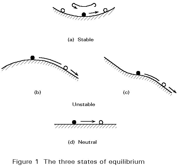
For rigid bodies, the stability can be illustrated by the well-known example of a ball on a curved plane (Figure 1). Resting on a concave surface (Figure 1a) the equilibrium is stable; if one gives the ball a small initial velocity, it will begin to oscillate but will remain in the close neighbourhood of its equilibrium state. On the other hand, if the system is not in a configuration of minimum V (potential energy), then an impulse leads to large deflections and velocities which develop very quickly, and the system is said to be unstable. This is the case where the ball rests on the crest of a convex surface (Figure 1b) or at a horizontal point of inflection of the surface (Figure 1c). If the ball rests on a horizontal plane, the equilibrium is called "neutral" (Figure 1d).
The intuitive example of the ball leads to the law of minimum potential energy of a system: "A conservative elastic system is in a state of stable equilibrium if, and only if, the value of the potential energy is a relative minimum".
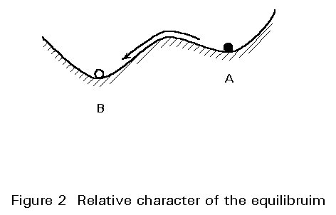
The words "relative minimum" are used because there may be other minima nearby at lower values of potential energy separated by small "hills" but the move from one minimum to another necessitates large disturbances (Figure 2). The existence of a relative minimum of the potential energy in the equilibrium configuration is, strictly speaking, only a sufficient condition for stability. However, this principle is, in practice, generally accepted as both a necessary and sufficient condition for stability.
It has been shown that the stability concept is related to potential energy of the system. However, stability of a static elastic system, or structure, may also be explained by stiffness considerations. Referring to Figure 1a, one can see that the derivative of the potential energy with respect to displacement gives the stiffness (in the figure, the slope of the surface) of the system.
Thus, positive stiffness implies a stable state, whereas at a stability limit the stiffness vanishes. For a structure, the stiffness is given in matrix form, which if it has both a positive and definite condition, guarantees a stable state for the structure. The point at which the state of a system changes from stable equilibrium into neutral equilibrium is called "the stability limit".
The system of a ball on a curved plane (where the stability depends only on the shape of the surface) can be compared to a structure such as a compressed column. In this case, the column may be stable or unstable, depending of the magnitude of the axial load, which is the controlling parameter of the system (Figure 3a). Since the member is initially straight and the load is axial, the structure will be in stable equilibrium for small values of N; if a disturbing force produces deflections, the column will return to its straight position. When the load reaches a certain level, called "critical load", the stable equilibrium reaches a limit. At this load Ncr, there exists another equilibrium position in a slightly deflected configuration of the column; if, at this load, the member is deflected by some small disturbance, it will not return to the straight configuration.
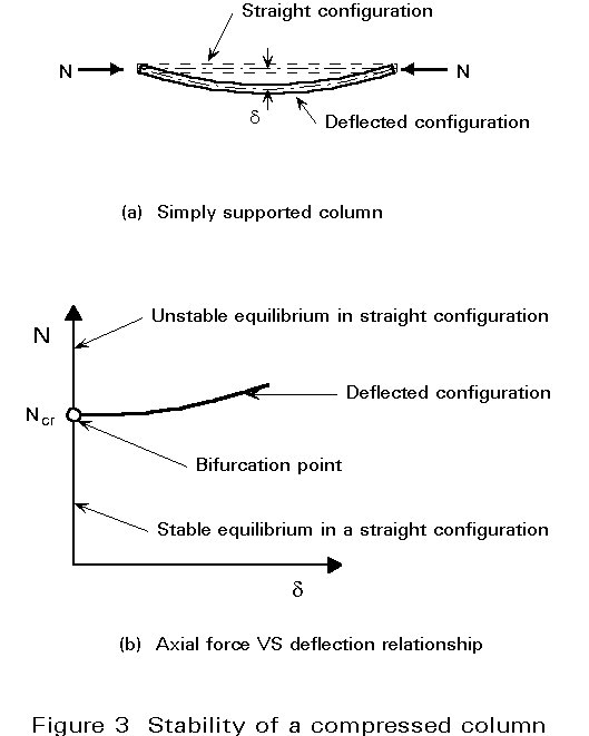
If the load exceeds the critical value, the straight position is unstable and a slight disturbance leads to large displacements of the member and, finally, to the collapse of the column by buckling. The critical point, after which the deflections of the member become very large, is called the "bifurcation point" of the system (Figure 3b).
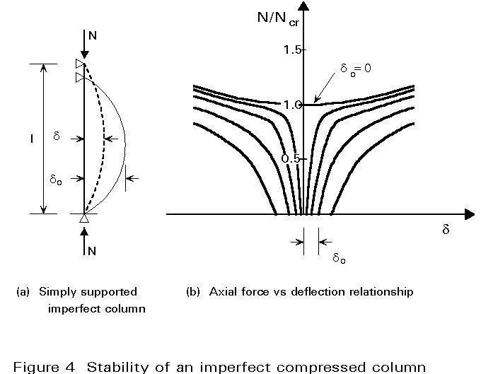
If the column is not initially perfectly straight, deflection starts from the beginning of the loading and there is no sudden buckling by bifurcation, but a continuous increase of the displacements (Figure 4). This phenomenon is called "divergence of the equilibrium" and there is no strict stability limit. If the material remains elastic, the stiffness of the column (given here by the slope of the N. d curve) is always positive but a small disturbance will produce very large displacements.
The reduction in the stiffness of a structural member is, in general, due to a change either in geometry or in mechanical properties. Stiffness reduction due to geometric change does not generally cause loss of stability but leads to large deflections. On the other hand, major stiffness reductions can result from the change in mechanical properties (yielding or fracture of material) and, in consequence, lead to collapse of the member. This important point is discussed in later lectures.
After the bifurcation point, three main situations can arise depending on the type of system under study (Figure 5). In Figure 5, N is the applied load, d is a displacement of one point of the system and x is the amplitude of the imperfection. Heavy solid lines in Figure 5 represent the equilibrium paths of the perfect system while light solid lines represent the equilibrium paths of imperfect systems, continuous lines representing stable equilibrium and dotted lined representing unstable equilibrium.
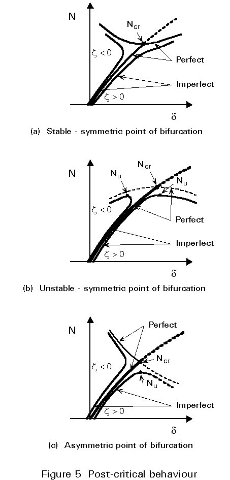
Small positive and negative imperfections have similar effects and yield a stable and rising equilibrium path. The buckling is characterized by a rapid growth of the deflections when the critical load of the perfect system is approached. This case is of great practical importance because columns, beams and plates show this type of postcritical behaviour.
The imperfections play an important role in modifying the behaviour of the system. Small imperfections of both signs induce a reduced load with regard to the critical load. This is, for example, the case in some systems composed of hinged bars.
For small positive values of the imperfection, the system loses its stability at a limit point (ultimate load), largely reduced by comparison to the critical point. On the other hand, small negative imperfections lead to a rising stable path. Here, the system is mainly sensitive to initial positive imperfections. This is, for example, the case in some trusses.
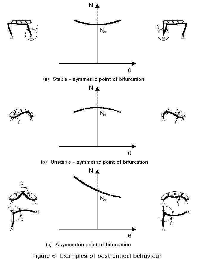
Figure 6 illustrates these three post-critical behaviours.
Buckling associated with bifurcation of equilibrium is not the only form of instability which can occur. In the case of shallow arches, shallow trusses and spherical domes, for example, snap-through buckling can occur where the initially stable path loses its stability when reaching the locally maximum value of the load, called the "limit point" of the system. This is shown in Figure 7a, which also shows that the response of an imperfect system is similar to that of the corresponding perfect system.
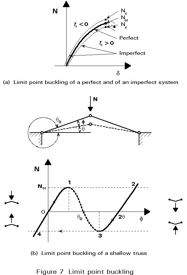
Figure 7b illustrates this buckling behaviour by considering a shallow truss made up of two hinged bars. When the load is first applied a stable path 0-1 is followed. At point 1, stability is lost and a dynamic jump through non-equilibrium states occurs from point 1 to 2 and the truss is now in an inverted position (snap-through). Point 2 also lies on a stable path and further loading may take place. For example, an unloading sequence follows the stable path from point 2 to 3 at which, once more, stability is lost causing the structure to jump dynamically from point 3 to 4. At point 4, the structure is on the original stable path and a new loading cycle can be started. This discussion shows that the dashed line between points 1 and 3, which represents the unstable equilibrium states, is totally inaccessible during the loading process.
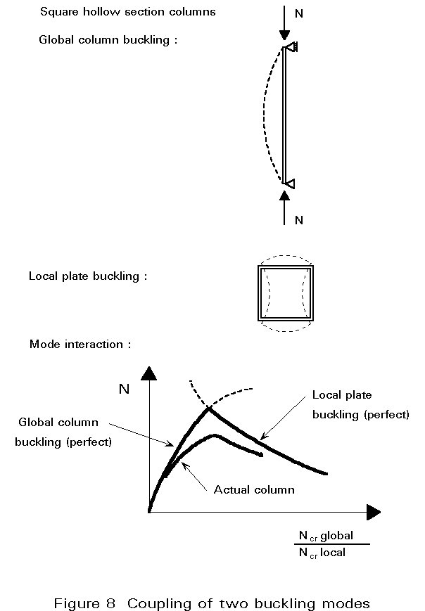
In some cases, structures can exhibit several instability modes at nearly the same critical loads or at critical loads which are very close. In these cases, called coupled bifurcations, the imperfections can lead to a significant reduction in the ultimate load compared to the ultimate loads of the single modes. Coupled bifurcation problems are generally difficult to analyse. Some coupled instabilities which can arise in steel structures and members are given below:
Figure 8 illustrates the reduction in the buckling load due to the coupling of a local and a global buckling mode as follows: